
20. Practices Recovery MD - 2023/24#
20.1. Citeseer dataset#
The citeseer dataset is a citation network dataset that contains scientific publications and their citations. The dataset consists of 3327 nodes and 4732 edges. Each node in the graph represents a scientific publication, and each edge represents a citation between two publications. The nodes are labeled with one of six classes, which correspond to the research areas of the publications.
In this section, we will load the citeseer dataset using Pytorch Geometric and explore its properties. We will visualize the graph, compute some basic statistics, and analyze its structure.
Let’s start by loading the Citeseer dataset using Pytorch Geometric.
import torch
from torch_geometric.datasets import Planetoid # Pytorch Geometric datasets
import torch_geometric.transforms as T # Pytorch Geometric transformations, in this case we are going to use the LargestConnectedComponents
from torch_geometric.utils import to_networkx # Convert PyG data object to NetworkX graph

# Load the Citeseer dataset
# root: root directory where the dataset should be saved
# name: name of the dataset
# transform: a function/transform that takes in an optional argument and returns a transformed version
dataset = Planetoid(root='data/Citeseer', name='Citeseer', transform=T.LargestConnectedComponents())
# Get the first element of the dataset, since it is a list of PyG data objects
data = dataset[0]
# Convert the PyG data object to a NetworkX graph
G = to_networkx(data, to_undirected=True)
# Get the labels of the nodes
labels = data.y.numpy()
print(f'Number of nodes: {G.number_of_nodes()}')
print(f'Number of edges: {G.number_of_edges()}')
print(f'Number of classes: {len(set(labels))}')
The code above loads the Citeseer dataset using Pytorch Geometric and converts it to a NetworkX graph. We then print the number of nodes, edges, and classes in the graph. Now let’s visualize the graph using NetworkX.
import matplotlib.pyplot as plt
plt.figure(figsize=(20, 15))
plt.title('Citeseer Dataset', fontsize=20)
pos = nx.kamada_kawai_layout(G)
# Color is based on data.y
colors = data.y.numpy()
nx.draw(G, pos=pos, cmap=plt.cm.viridis, node_color=colors, node_size=50, edge_color='black', width=0.7, with_labels=False, node_shape='o', alpha=0.8)
plt.show()
Giving us the following graph:
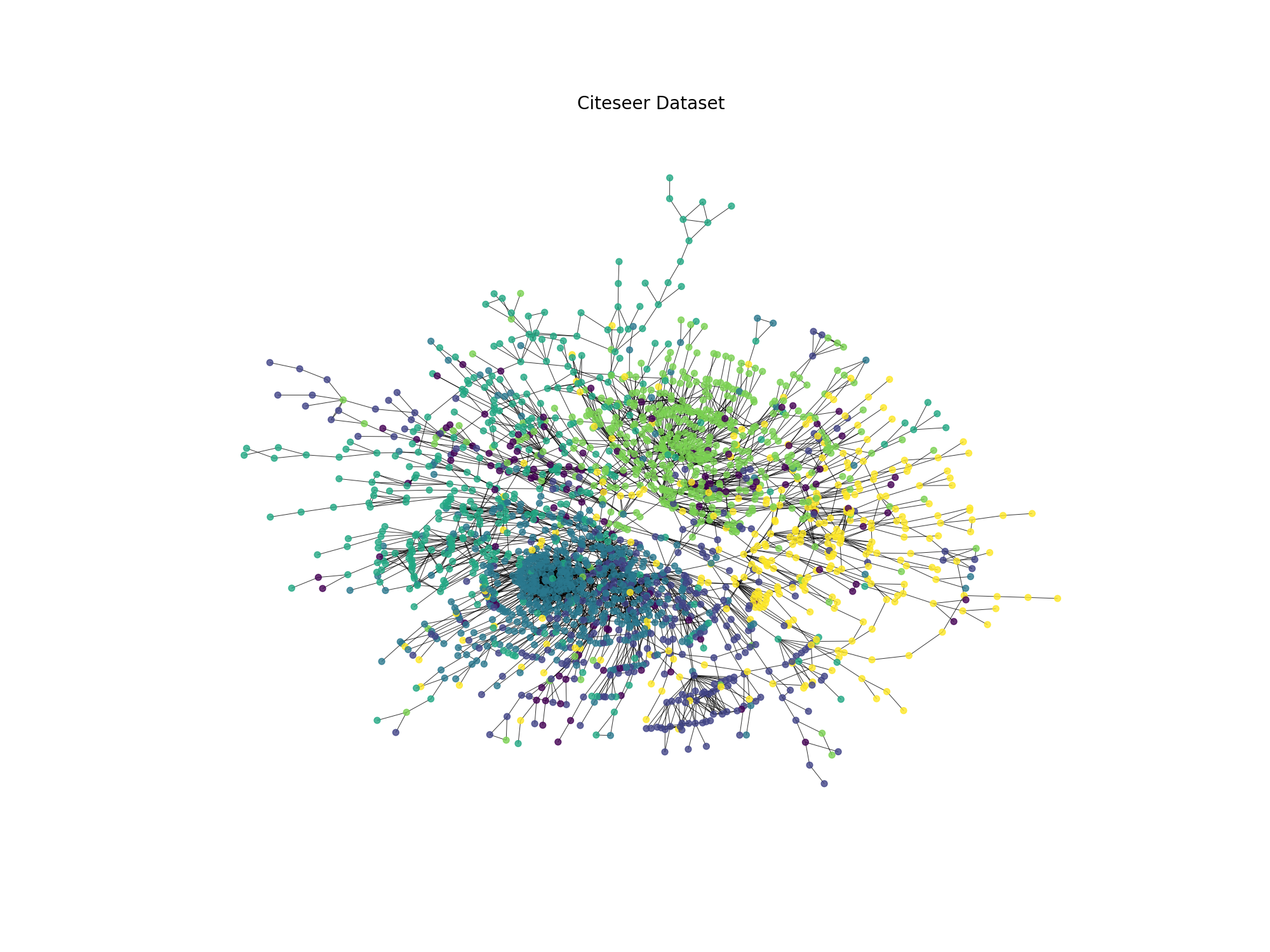
Fig. 20.1 Citeseer dataset visualization#
20.1.1. Node2Vec algorithm#
Following the idea of Word2Vec, the Node2Vec algorithm is a representation learning algorithm that is used to learn the embeddings of the nodes in a graph. The embeddings of the nodes are learned in such a way that the nodes that are close in the graph are also close in the embedding space.
Here is a brief explanation of how the Node2Vec algorithm works:
Generate random walks: The first step of the Node2Vec algorithm is to generate random walks on the graph. The random walks are generated by starting at a given node in the graph and then moving to a neighboring node with a certain probability. The random walk continues in this way until it reaches a terminal node.
Learn the embeddings: The second step of the Node2Vec algorithm is to learn the embeddings of the nodes in the graph. The embeddings of the nodes are learned in such a way that the nodes that are close in the graph are also close in the embedding space. The embeddings are learned using the Skip-Gram model, which is a variant of the Word2Vec model.
20.1.1.1. Code snippet#
Here is a code snippet that shows how to use the Node2Vec algorithm to learn the embeddings of the nodes in a graph:
import numpy as np
import networkx as nx
from gensim.models import Word2Vec

# Función para realizar una caminata aleatoria en el grafo
def node2vec_walk(G, start_node, walk_length):
    walk = [start_node]
    while len(walk) < walk_length:
        cur_node = walk[-1]
        neighbors = list(G.neighbors(cur_node))
        if len(neighbors) > 0:
            walk.append(np.random.choice(neighbors))  # Selecciona un vecino al azar
        else:
            break
    return walk

# Función para generar múltiples caminatas aleatorias desde cada nodo del grafo
def generate_walks(G, num_walks, walk_length):
    walks = []
    nodes = list(G.nodes())
    for _ in range(num_walks):
        np.random.shuffle(nodes)  # Mezcla los nodos para añadir aleatoriedad
        for node in nodes:
            walks.append(node2vec_walk(G, node, walk_length))  # Genera una caminata aleatoria desde el nodo
    return walks

# Función principal de Node2Vec
def node2vec(G, dimensions, num_walks, walk_length):
    walks = generate_walks(G, num_walks, walk_length)  # Genera todas las caminatas aleatorias
    walks = [list(map(str, walk)) for walk in walks]  # Convierte los nodos a cadenas para gensim
    # walks: Lista de caminatas aleatorias
    # vector_size=dimensions: Tamaño del vector de embeddings
    # window=5: Tamaño de la ventana de contexto, en nodos seria 5 nodos a la izquierda y 5 nodos a la derecha
    # workers=2: Número de hilos para entrenar el modelo
    model = Word2Vec(walks, vector_size=dimensions, window=5, workers=2)  # Entrena el modelo Word2Vec con las caminatas aleatorias
    return model
20.1.2. Exercise 0#
In the following two exercises, it is compulsory to add a discussion of the results. And very extensive explanations of the parameters that you modified and how they affected the performance of the classifier. If you don’t do this, you will get a 0 in the exercise.
20.1.3. Exercise 1#
In the previous section, we learned how to use Node2Vec to generate node embeddings for a graph. Now, we will use the node embeddings to perform node classification on the Cora dataset. We will train a simple logistic regression classifier on the node embeddings to predict the class labels of the nodes.
The steps to perform node classification are as follows:
Generate node embeddings using Node2Vec.
Train a logistic regression classifier on the node embeddings. Note that you will need to split the dataset into training and test sets (60% training, 40% test).
Evaluate the classifier on the test set. You will need to run the training and evaluation 10 times and calculate the average accuracy to get a more reliable estimate of the classifier’s performance. If you don’t do this, you will get a 0 in the exercise.
Report the average accuracy of the classifier, and discuss the results. In the discussion, I want to see all the parameters that you modified during the process (e.g., the number of walks, the length of the walks, the embedding dimension, etc.) and how they affected the performance of the classifier. If you put a very long explanation of the parameters that you modified and how they affected the performance of the classifier, you will get a 10 in the exercise, without taking into account the accuracy of the classifier.
Note
Important: You need to save the accuracy of each run in a csv file called node_classification_results_yourname.csv and upload it to the platform.
Important: In the csv file at least should contain 6 configurations of the Node2Vec algorithm and the accuracy of the classifier for each configuration(with a pandas shape of 6 rows representing each configuration and 5 colummns representing the configuration, accuracy and std). If you don’t do this, you will get a 0 in the exercise.
Note
Important: It is forbidden to change the classifier model. Also it is important to initialize the classifier with different random states each time you run the training and evaluation to ensure that the classifier is trained on different data each time. If you don’t do this, you will get a 0 in the exercise.
You can use the following code as a reference:
# Now let's try to classify the nodes using the embeddings
from sklearn.model_selection import train_test_split
from sklearn.linear_model import LogisticRegression
from sklearn.metrics import accuracy_score
# Split the data into training and test sets
X = embeddings
y = data.y.numpy()
X_train, X_test, y_train, y_test = train_test_split(X, y, test_size=0.4, random_state=0)

# Train a logistic regression classifier
clf = LogisticRegression(max_iter=1000, random_state=0)
clf.fit(X_train, y_train)

# Evaluate the classifier
y_pred = clf.predict(X_test)
accuracy = accuracy_score(y_test, y_pred)
print(f'Accuracy: {accuracy:.2f}')
Note
Important: You will need to run the training and evaluation 10 times and calculate the average accuracy to get a more reliable estimate of the classifier’s performance. If you don’t do this, you will get a 0 in the exercise.
Note
Important: You need to change the random_state in the train_test_split function to a different value each time you run the training and evaluation to ensure that the data is split differently each time. If you don’t do this, you will get a 0 in the exercise.
#### The resulting report should be saved in a csv file called node_classification_results_yourname_ex1.csv and with this format:
Configuration |
Accuracy |
Std |
Number of walks |
Length of walks |
Embedding dimension |
|---|---|---|---|---|---|
Configuration 1 |
—- |
—- |
{number} |
{length} |
{dimension} |
Configuration 2 |
—- |
—- |
{number} |
{length} |
{dimension} |
Configuration 3 |
—- |
—- |
{number} |
{length} |
{dimension} |
Configuration 4 |
—- |
—- |
{number} |
{length} |
{dimension} |
Configuration 5 |
—- |
—- |
{number} |
{length} |
{dimension} |
Configuration 6 |
—- |
—- |
{number} |
{length} |
{dimension} |
20.2. Message Passing#
In the previous section, we have seen how to use node2vec to generate node embeddings. In this section, we will use the message passing (not neural message passing) to generate node embeddings. The message passing is a technique to propagate information between nodes in a graph. The message passing is a fundamental concept in graph neural networks.
The message passing is defined as follows:
Each node sends a message to its neighbors.
Each node aggregates the messages from its neighbors.
Each node updates its own state based on the aggregated messages.
In a mathematical form, the message passing can be defined as follows:
where \(h_v^{(l)}\) is the state of node \(v\) at layer \(l\), \(\mathcal{N}(v)\) is the set of neighbors of node \(v\), and \(\text{AGGREGATE}^{(l)}\) is the aggregation function at layer \(l\). The aggregation function can be a sum, mean, max, etc. If we use the sum aggregation function, the message passing can be defined as follows:
And in matrix form, the message passing can be defined as follows:
where \(H^{(l)}\) is the state matrix at layer \(l\), \(A\) is the adjacency matrix, and \(H^{(l+1)}\) is the state matrix at layer \(l+1\). The message passing can be applied multiple times to generate node embeddings. The node embeddings can be used for node classification, link prediction, etc.
20.2.1. Exercise 2#
In the previous section, we learned how to use node2vec and in this section, we learned how to use the message passing to generate node embeddings. Now, we will combine the node2vec and message passing to generate node embeddings. You just have to concatenate the node embeddings generated by node2vec and message passing. Then, you will train a logistic regression classifier on the concatenated node embeddings to predict the class labels of the nodes. You need to follow the same steps as in Exercise 1.
Note
Important: What I want to see in the discussion is how the combination of node2vec and message passing affected the performance of the classifier. It is also important to mention that you can perform the message passing multiple times, for instance 3 times. Therefore, you will have to concatenate the node embeddings generated by node2vec and message passing 3 times and generate a report with the average accuracy of the classifier, the std, node2vec parameters, and message passing parameters.
#### The resulting report should be saved in a csv file called node_classification_results_yourname_ex2.csv and with this format:
Configuration |
Accuracy |
Std |
Node2Vec Parameters |
Message Passing Parameters |
|---|---|---|---|---|
Configuration 1 |
—- |
—- |
{parameters} |
{parameters} |
Configuration 2 |
—- |
—- |
{parameters} |
{parameters} |
Configuration 3 |
—- |
—- |
{parameters} |
{parameters} |
20.3. Submission#
For the delivery of the practices, you must submit the following files:
notebook_practices_yourname.ipynb: Jupyter notebook with the development of the exercises.node_classification_results_yourname_ex1.csv: CSV file with the results of Exercise 1.node_classification_results_yourname_ex2.csv: CSV file with the results of Exercise 2.