19. Real cases dataset

In this section, we will work with a real-world dataset to apply the concepts we have learned in the previous sections. So, before we dive into this exploration, it is important to make a recap of what we have already seen in previous classes. And understand the importance of the concepts we have learned so far.

19.1. Pytorch Geometric

Pytorch Geometric is a library for deep learning on irregular input data such as graphs. It consists of various methods and utilities to process graphs and extract information from them. The library is built on top of Pytorch, which is a popular deep learning library. Pytorch Geometric provides a lot of tools to work with graphs, such as creating graphs, loading datasets, and applying different models to them.

Also PyG provides a lot of datasets that can be used to test the models in different tasks such as node classification, link prediction, graph classification, etc. In this section, we will use one of the datasets provided by PyG to create a graph and explore it.

For more details about Pytorch Geometric, you can check the official documentation here.

19.2. Cora dataset

Fig. 19.1 Cora source

The Cora dataset is a citation network dataset that contains scientific publications and their citations. The dataset consists of 2708 nodes and 5429 edges. Each node in the graph represents a scientific publication, and each edge represents a citation between two publications. The nodes are labeled with one of seven classes, which correspond to the research areas of the publications.

In this section, we will load the Cora dataset using Pytorch Geometric and explore its properties. We will visualize the graph, compute some basic statistics, and analyze its structure.

Let’s start by loading the Cora dataset using Pytorch Geometric.

import torch
from torch_geometric.datasets import Planetoid # Pytorch Geometric datasets
import torch_geometric.transforms as T # Pytorch Geometric transformations, in this case we are going to use the LargestConnectedComponents
from torch_geometric.utils import to_networkx # Convert PyG data object to NetworkX graph

# Load the Cora dataset
# root: root directory where the dataset should be saved
# name: name of the dataset
# transform: a function/transform that takes in an optional argument and returns a transformed version
dataset = Planetoid(root='data/Cora', name='Cora', transform=T.LargestConnectedComponents())
# Get the first element of the dataset, since it is a list of PyG data objects
data = dataset[0]
# Convert the PyG data object to a NetworkX graph
G = to_networkx(data, to_undirected=True)
# Get the labels of the nodes
labels = data.y.numpy()
print(f'Number of nodes: {G.number_of_nodes()}')
print(f'Number of edges: {G.number_of_edges()}')
print(f'Number of classes: {len(set(labels))}')

The code above loads the Cora dataset using Pytorch Geometric and converts it to a NetworkX graph. We then print the number of nodes, edges, and classes in the graph. Now let’s visualize the graph using NetworkX.

import matplotlib.pyplot as plt
plt.figure(figsize=(20, 15))
plt.title('Cora Dataset', fontsize=20)
pos = nx.kamada_kawai_layout(G)
# Color is based on data.y
colors = data.y.numpy()
nx.draw(G, pos=pos, cmap=plt.cm.viridis, node_color=colors, node_size=50, edge_color='black', width=0.7, with_labels=False, node_shape='o', alpha=0.8)
plt.show()

Giving us the following graph:

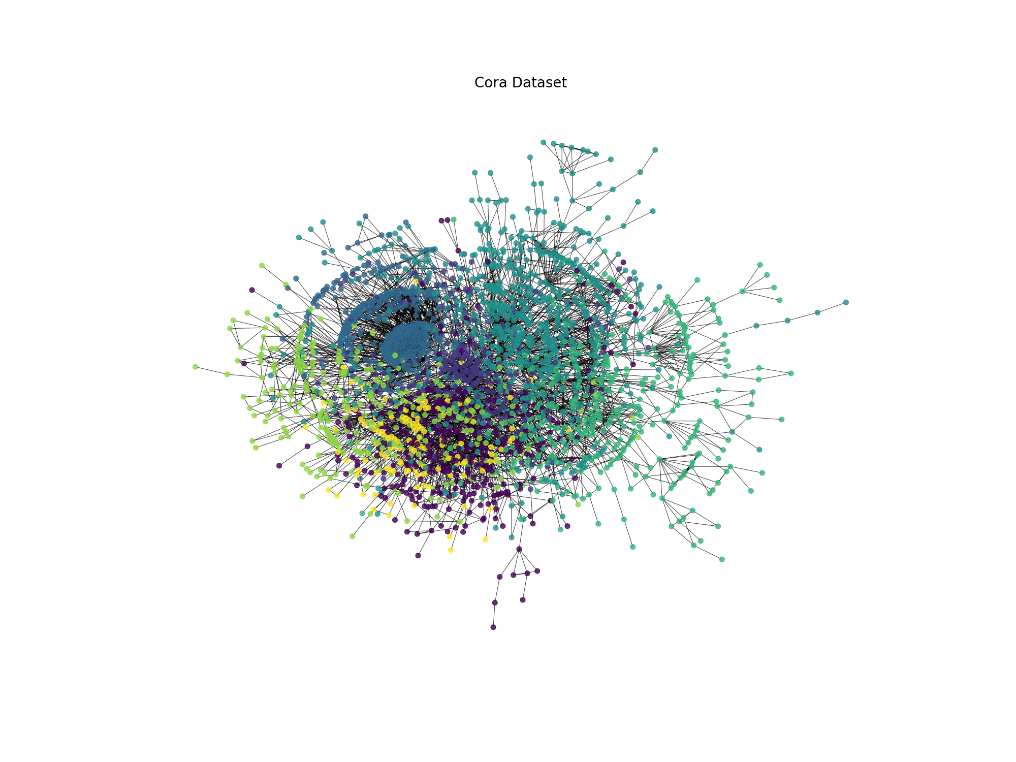
Fig. 19.2 Cora dataset visualization

The graph represents the Cora dataset, where each node is colored according to its class label. The graph is a citation network, where nodes represent scientific publications and edges represent citations between publications. The colors represent the research areas of the publications.

19.3. Exercises

19.3.1. Exercise 1

In the previous section, we learned how to use Node2Vec to generate node embeddings for a graph. Now, we will use the node embeddings to perform node classification on the Cora dataset. We will train a simple logistic regression classifier on the node embeddings to predict the class labels of the nodes.

The steps to perform node classification are as follows:

1. Generate node embeddings using Node2Vec.

2. Train a logistic regression classifier on the node embeddings. Note that you will need to split the dataset into training and test sets (60% training, 40% test).

3. Evaluate the classifier on the test set. You will need to run the training and evaluation 10 times and calculate the average accuracy to get a more reliable estimate of the classifier’s performance. If you don’t do this, you will get a 0 in the exercise.

4. Report the average accuracy of the classifier, and discuss the results. In the discussion, I want to see all the parameters that you modified during the process (e.g., the number of walks, the length of the walks, the embedding dimension, etc.) and how they affected the performance of the classifier. If you put a very long explanation of the parameters that you modified and how they affected the performance of the classifier, you will get a 10 in the exercise, without taking into account the accuracy of the classifier. Important: You need to save the accuracy of each run in a csv file called node_classification_results_yourname.csv and upload it to the platform. Important: In the csv file at least should contain 24 configurations of the Node2Vec algorithm and the accuracy of the classifier for each configuration(with a pandas shape of 24 rows representing each configuration and 5 colummns representing the configuration, accuracy and std). If you don’t do this, you will get a 0 in the exercise.

Note

Important: It is forbidden to change the classifier model. Also it is important to initialize the classifier with different random states each time you run the training and evaluation to ensure that the classifier is trained on different data each time. If you don’t do this, you will get a 0 in the exercise.

You can use the following code as a reference:

# Now let's try to classify the nodes using the embeddings
from sklearn.model_selection import train_test_split
from sklearn.linear_model import LogisticRegression
from sklearn.metrics import accuracy_score
# Split the data into training and test sets
X = embeddings
y = data.y.numpy()
X_train, X_test, y_train, y_test = train_test_split(X, y, test_size=0.4, random_state=0)

# Train a logistic regression classifier
clf = LogisticRegression(max_iter=1000, random_state=0)
clf.fit(X_train, y_train)

# Evaluate the classifier
y_pred = clf.predict(X_test)
accuracy = accuracy_score(y_test, y_pred)
print(f'Accuracy: {accuracy:.2f}')

Note

Important: You will need to run the training and evaluation 10 times and calculate the average accuracy to get a more reliable estimate of the classifier’s performance. If you don’t do this, you will get a 0 in the exercise.

Note

Important: You need to change the random_state in the train_test_split function to a different value each time you run the training and evaluation to ensure that the data is split differently each time. If you don’t do this, you will get a 0 in the exercise.

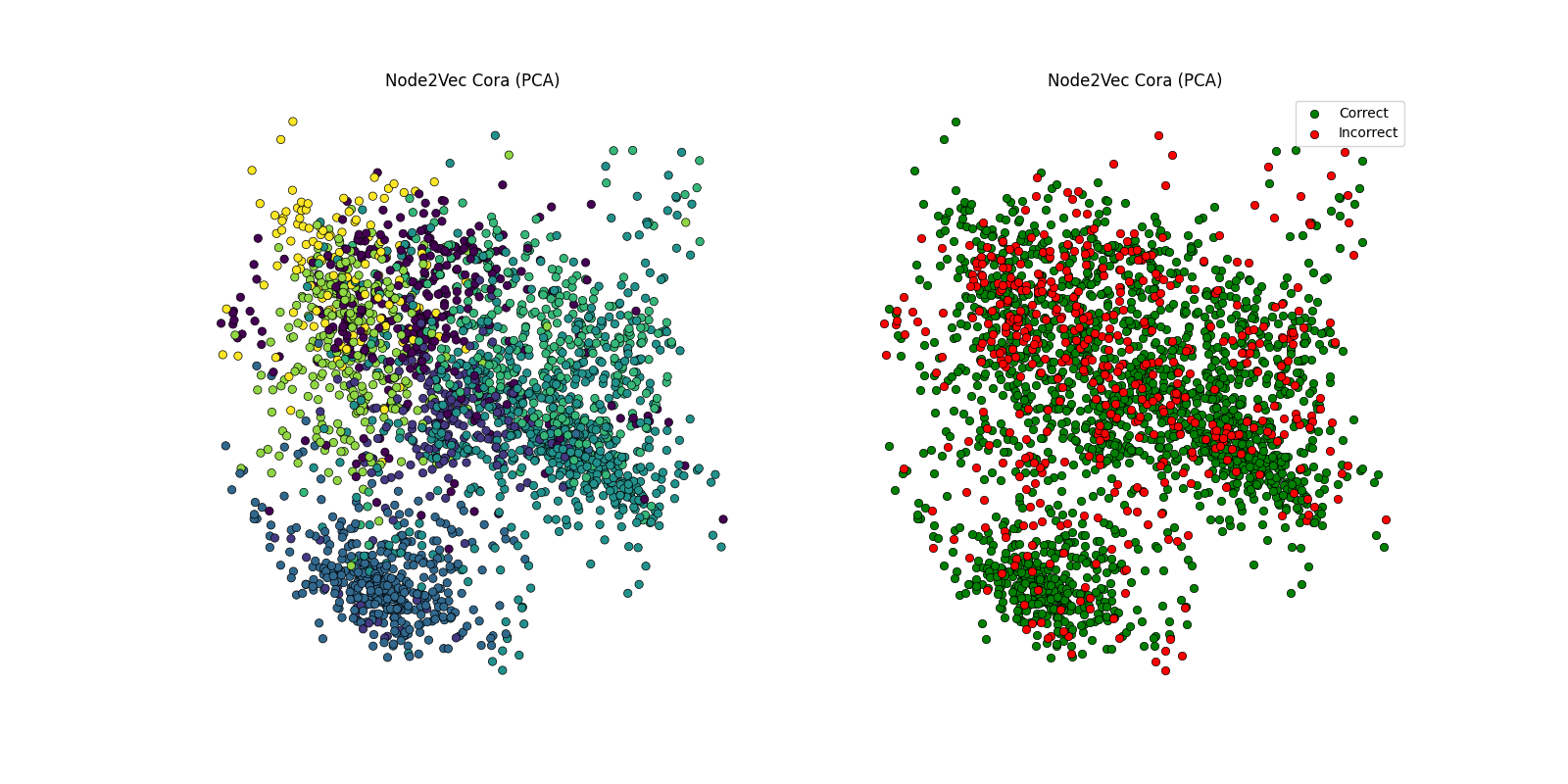
Fig. 19.3 Disscussion of the results in visual form