
4. Random walks on graphs#
4.1. Markov chains#
So far, we have studied both independent random processes and conditional random processes. In this regard, when we have independence, our random process is a simple random walk (see RWrand). However, when the variables in the random process are fully conditioned, the corresponding random process is more difficult to study unless we have a martingale. Fortunately, there is something in between the simplicity of independent random processes and the full conditioning of the martingale: we refer to Markov chains.
Markov chain. A sequence of random variables \(X_0,X_1,\ldots\) is a Markov chain if for all possible states (values of the random variables) \(x_{t+1},x_{t},\ldots,x_1\) we have:
i.e. the probability of a future event only depends on that of a present one. This is called the Markov property or the memoryless property.
A couple of interesting properties:
Irreducibility. We say that a state \(j\) in the Markov chain (MC) is accesible from another state \(i\) if exists \(t\ge 0\) so that
that is, we can get from a state \(i\) to state \(j\) in \(t\) steps with probability \(p_{ij}(t)\). Then, a MC is irreducible if each pair \((i,j)\) of states is mutually accessible.
Periodicity. A state \(i\) has period \(d_i\) if
where \(\text{gcd}\) denotes the greatest common divisor. Then, if \(d_i>1\) the state \(i\) is periodic; it \(d_i=1\) it is aperiodic. Then a MC is aperiodic if all states have period \(d_i=1\).
Graphs. A graph \(G=(V,E)\) consists of a set of nodes or vertices \(V={1,2,\ldots,n}\) where \(|V|=n\), and a set of edges \(E\subseteq V\times V\).
An edge \(e=(i,j)\) is denoted by a pair of nodes \(i\) and \(j\), where \(i\) is the origin and \(j\) the target or destination.
If the graph is undirected both \((i,j)\) and \((j,i)\) do exist for all \(e\in E\). Otherwise, the graph is directed.
If \(e=(i,i)\) we have a self-loop.
Graphs are very flexible mathematical tools. We commence by using them for describing a random process. The nodes \(V\) provide the states and the edges \(E\) provide the transitions between states. Actually we label the edges with the probability of a Markovian transition \(p(j|i) = p_{ij}\).
The following example is motivated by the essay Random Walks and Electric Networks by Doyle and Snell.
We want to build a graph for the drunkard’s walk. A man walks along a \(5-\)blocks stretch in Madison Avenue. He starts at corner \(x\) and, with probability \(1/2\) walks one block to the right and, also with probability \(1/2\) walks one block to the left. At the next corner, he again choses his direction randomly. He continues until he reaches corner \(5\), which is home, or corner \(0\), which is a bar. In both latter cases he stays there.
Our graph for this walk has \(n=6\) vertices or states \(V=\{0,1,2,3,4,5\}\), where \(5\) is \(\text{Home}\) and \(0\) is the \(\text{Bar}\). See Drunk where the edges or transitions are in blue (bidirectional if we no depict the arrowheads) and the possible decision for node \(x=3\) are depicted in black.
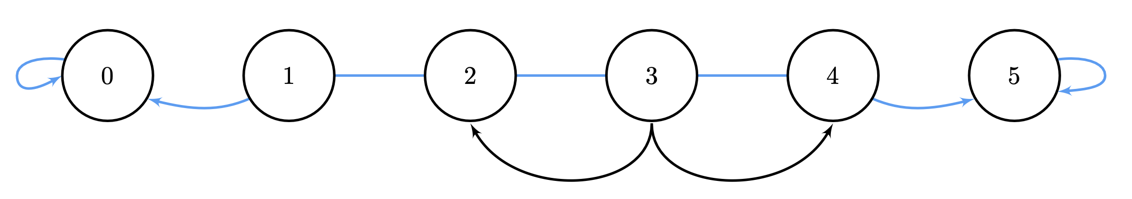
Fig. 4.1 A graph for the drunkard’s walk.#
Actually, the edges of the above graph are \(E=\{(0,0),(1,0),(1,2),(2,1)\ldots,(4,5),(5,5)\}\)
Why our graph mimics the drunkard’s walk, and why it is a MC?
We have two states, \(0\) and \(1\), with self-loops and no edges for returning to any other node. These states are called absorbing states in the MC terminology, since once the Markov-chain-random walk (MCRW) reaches them, it is trapped there. As a result the MC is reducible.
The graph is almost bipartite, i.e. we can parition \(V\) in to subsets \(V_1=\{0,2,4\}\) and \(V_2=\{1,3,5\}\) so that nodes in \(V_1\) can only go nodes of \(V_2\) (except the absorbing nodes) and viceversa. As a result, the MC is almost aperiodic. Non-absorbing nodes have period \(2\) and the absorbing ones have period \(1\).
If we start our MCRW at a non-absorbing state, say \(x\in\{2,3,4\}\) we walk left with probability \(1/2\) and right also with probability \(1/2\).
The degree \(\text{deg}(i)\) of a node \(i\) in the graph is the number of neighbors \({\cal N}_i\), i.e. the number of outgoing edges from \(i\). In our graphs we have that all non-absorbing nodes have degree \(2\) whereas the absorbing states have degree \(1\) (actually their neighbors are themselves).
The degree \(\text{deg}(i)\) of each node \(i\) reveals that the (Markovian) probability of making a transition to a neighbor is
and \(a_{ij}=1\) means that nodes \(i\) and \(j\) are adjacent. For absorbing states, we have \(a_{ij}=0\;\forall j\neq i\). As a result, for these states \(p_{ii}=1\) and \(p_{ij}=0\) for \(j\neq i\).
Patterns of the drunkard’s walk. In order to have a rough idea of the behavior of this Markov process, we have generated \(40,000\) random walks (\(10,000\) starting at each non-absorbing states \(x=1,2,3,4\)). Each random walk has length \(l=10\). Why? We will discover that shorly. What is important now is to note that some of the walks end up in one of the absorbing states (\(x=0\)), whereas many others end in the other one (\(x=5\)). The probability of reaching each absorbing state is \(1/2\).
We plot these walks in Drunkard. The darkest the blue line, the slower the walk reaches \(x=5\). This means that if the walks reaches \(x=5\) at the maximum length of the path \(l=10\) it becomes the darkest one.
Some iteresting patterns:
As we start uniformly the same number of paths at each non-absorbing state, there is no clear difference between the paths ending in \(x=0\) and those ending in \(x=5\).
In addition, some paths tending to \(x=0\) turn suddenly towards \(x=5\) and vice versa.
Apparently, all the non-absorbing states reach \(x=5\) equally slowly. However this is misleading. Actually, most of the paths reach \(x=5\) very early. This suggests that the probability of reaching \(x=5\) from any non-absorbing state is not uniform. This leads us to the answer the first question to solve about a random walk: what is the probability of ending \(\text{Home}\).
4.2. Recurrence relations#
Before addressing the two fundamental questions for a MCRW: (a) where does it converge to, and (b) how long does it take, it is important to note that the remainder of this section requires some practice with algebraic solvers of recurrent relations, namely linear difference equations. They are very practical tools that are explained in the excellent Github of Mathew Aldridge and even in the Wikipedia. The examples below have been adapted from the first source and solve some of the exercises in Random Walks and Electric Networks by Doyle and Snell.
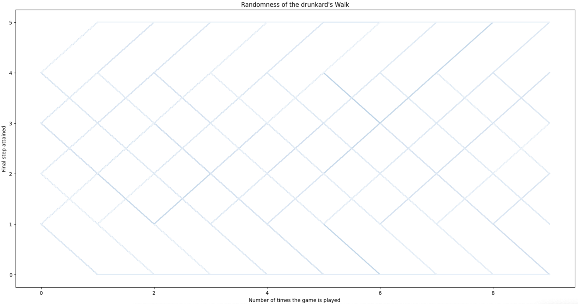
Fig. 4.2 Patterns of generated drunkard’s walks.#
Q1. What is the probability of ending at \(\text{Home}\) if we start from the non-absorbing state \(x\)?
In other words, what is the probability of hitting \(x=5\) from \(x\) before hitting \(x=0\)?
We commence by formulating the Markovianity of the drunkward’s path in a more generic way:
where: \(x_{n}\) is the position of the walk at step \(n\), \(p = 1 - q = 1/2\) is the probability of a transition from a non-absorbing state and \(m=5\) is the target node.
We pose the above formula in probabilistic terms using the condition on the first step:
Herein, we use the theorem of total probability for the following events:
Then, total probability means that the probability of an event given two (or more) exclusive events is
In our case:
and we want to calculate both \(p(E|A)\) and \(p(E|\bar{A})\) to calculate \(P(E)\).
Formulate and solve a recurrence relation:
Then, we have to solve the following recurence relation:
where \(r_0 = 0\) and \(r_m=1\) are the boundary conditions that specify success if we reach \(m\) (\(\text{Home}\)) and failure if we reach \(0\) (\(\text{Bar}\)).
We formulate the recurrence relation as a linear difference equation. In this case it is homogeneous (like an homogeneous linear system \(\mathbf{A}\mathbf{x}=\mathbf{0}\)) since:
First of all, we apply the following change of variable:
which leads to
and taking \(\lambda^{n-1}\) as common factor yields
where \(p\lambda^{2} + q - \lambda = 0\) is the characteristic equation of the recurrence. Then, reorganzing the coefficients we have \(p\lambda^{2} - \lambda + q = 0\). To solve this quadratic equation is convenient to use the remainder theorem (Ruffini). The dividers of the independent term (\(q\)) are \(\pm 1\) and \(\pm q\). If we try first \(+1\), and apply \(q = 1-p\), this leads to the equation \(\lambda p - q = 0\) with yields \(\lambda =\frac{q}{p}\) tha we call \(\rho\). Then, the factorization we are looking for is
Now, we have two cases:
If \(\rho \neq 1\), then we have two distinct roots. In this case, the general solution of an homogeneous equation has the shape:
In order to determine \(A\) and \(B\) we exploit the two boundary conditions \(r_0=0, r_m=1\):
From \(A + B = 0\) we get \(A = -B\) which leads to
and, as a result
If \(\rho=1\) we have \(p=q\) and this means that we have two repeated solutions \(\lambda_1=\lambda_2 = 1\). In this case, the general solution has the following shape:
which leads to
whose solutions are \(A = 0\) and \(B = \frac{1}{m}\).
Finally
The generic result is:
Result for the ubiased walk. If \(p=q=1/2\) we have a random process according to the graph in Drunk. The probability of getting \(\text{Home}\), i.e. of hitting \(x=m=5\) before hitting \(x=0\) is \(p(x)=\frac{x}{m} = \frac{x}{5}\). The closer we are to \(\text{Home}\) the more probable is that we get there. Note that if we invert the boundary conditions priming going to the \(\text{Bar}\), the probability of getting there before arriving home is \(p(x)=1-\frac{x}{5}\).
However, as \(m\rightarrow\infty\) the probability of getting \(\text{Home}\) tends to zero, i.e. \(p(x)\rightarrow 0\).
The result for the unbiased (fair) walk is consistent with our observations in Drunkard and shows that the probability of reaching \(\text{Home}\) is not uniform. This result also explain why most of the \(40,000\) random walks lauched uniformly from any of the non-absorbing states reach \(\text{Home}\) very soon.
Result for the biased walk. Biased walks, however, are modeled in a different way. We label the edges with their probabilities. Then, instead of getting the transition probabilities from the degree, we simply set \(p_{ij}=a_{ij}p\) or \(p_{ij} = a_{ij}q\) as in Drunkpq
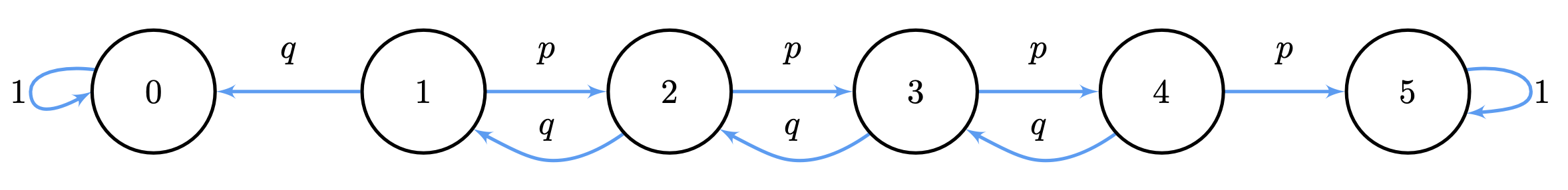
Fig. 4.3 Graph for biased drunkard’s walks.#
If \(q\ll p\), then \(p(x)\rightarrow 1\) since we are drifted to the right. Symmetrically, if \(q\gg p\), then \(p(x)\rightarrow 0\) since \(m>n\).
As \(m\rightarrow\infty\), we have that \(p(x)\rightarrow 0\), independently of the relationship between \(p\) and \(q\) since
In Drunkardpq where \(p=0.25, q=0.75\) we can see that few walks reach \(x=5\), actually the proportion of “successful” paths is \(p\).
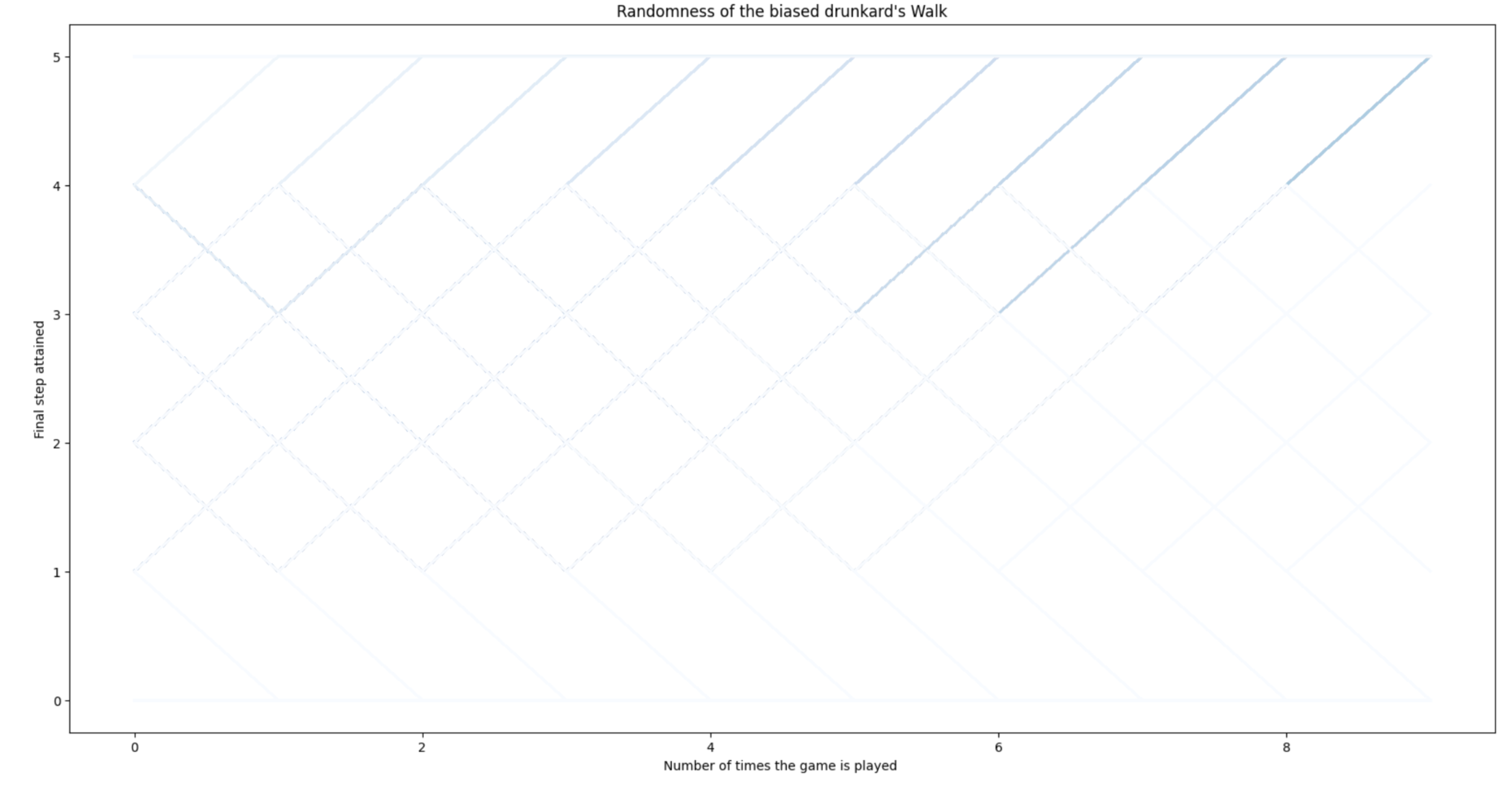
Fig. 4.4 Patterns of generated biased drunkard’s walks with \(p=0.25\).#
Q2. What is the expected time or hitting time for arriving \(\text{Home}\) if we start from the non-absorbing state \(x\)?
We are interested in estimating the expected hitting time of \(x=5\).
As before, we rely on linear difference equations.
We pose the above formula in probabilistic terms using the condition on the first step:
Herein, we use the conditional expectations for the following random variables:
where \(Y\) has values \(y=\text{left}\) and \(y=\text{right}\).
Then,
However, we are interested in \(E(X)\), which is defined by the tower property of conditional expectation:
where \(Y\) is the outcome of the first step.
In this regard,
Always count \(1\) because we had made a step.
This leads us to the following inhomogeneous recurrence relation:
and we have
Whose left-hand-size lhs leads to the same homogeneous recurrence equation that we have studied before.
If \(\rho\neq 1\) the general solution (\(\lambda_1=1, \lambda_2=\rho\) are solutions of the homogeneous version) has the shape
Since we need a particular solution for the full equation and the lhs is a constant, we start trying to set \(d_{n}=C\):
Next, we try with \(d_{n}=Cn\):
i.e. \(C = \frac{-1}{p-q}\) and the particular solution becomes
Then we apply the boundary conditions \(d_0=0, d_m=0\) to find \(A\) and \(B\):
\(A = - B\) and \(-B + B\rho^m = \frac{m}{p-q}\Rightarrow (\rho^m -1)B = \frac{m}{p-q}\Rightarrow B = \frac{1}{\rho^m-1}\cdot\frac{m}{p-q}\;.\)
Then
If \(\rho = 1\), i.e \(p=q=1/2\), the general solution (\(\lambda_1=1, \lambda_2=1\) are solutions of the homogeneous version) has the shape
For getting a particular solution we find that both the eductated guesses (antsazs) \(d_i=C\) and \(d_i= nC\) do not work. We try \(d_i=n^2C\):
and the resulting general solution is:
Then, we exploit again the the boundary conditions \(d_0=0, d_m=0\) to find \(A\) and \(B\):
And for \(A=0, B=m\) the general solution is
which clearly tells us that the hitting time of \(n\) is \(O(n^2)\) por \(p=q=1/2\) since we have equal probability of go back and forth.
Summarizing
Result for the ubiased walk. If \(p=q=1/2\) the hitting time of \(x=m\) from \(n\) is \(O(n^2)\) since we have equal probability of go back and forth.
The behavior for \(m\rightarrow\infty\) is obvious:
since \(m\) becomes impossible to be reached from \(n\).
Result for the biased walk. If \(p\neq q\) and \(p\ll q\), the walk is drifted to the left and this means that \(\rho\gg 1\), \(m\) is amplified and the hitting time from \(n\) increases notably. However, if \(p\gg q\), \(m\) is attenuated and this reduces the hitting time from \(n\).
Actually, the behavior for \(m\rightarrow\infty\) is:
We have two cases:
If \(q>p\), then \(\rho^m\gg m\) and \(\lim_{m\rightarrow\infty}\frac{1}{p-q}\left(m\frac{\rho^n}{\rho^m}-n\right)\) = \(\frac{1}{p-q}(-n)= \frac{1}{q-p}(n)\). Then, the hitting time is a fraction of \(n\).
If \(p>q\), then \(\rho^m\ll m\) and \(m\) is amplified wrt \(n\), increasing the hitting time.
Gambler’s ruin. The drunkard walk can be also interpreted in terms of the classical model of the Gambler’s ruin. The idea is as follows.
We have two players, Alice and Bob, starting respectively with \(a\) and \(b\) dollars, where \(a + b = m\).
They bet \(1\) dollar at each step.
Alice wins with probability \(p\) and Bob wins with probability \(q\), where \(p + q = 1\). Winning implies increasing the personal fortune by \(1\) taking it from the other’s fortune, i.e. if Alice wins the first round, the state of their respective fortunes are \((a+1,b-1)=m\). If Bob does, the state is \((a-1,b+1)=m\).
Therefore, reaching \(0\) means that Alice is ruined whereas reaching \(m\) means that Bob is ruined. In both cases we stop the game.
Exercise. Gambler’s ruin can be slightly modified to become a variant of a Birth-death chain. Suppose that we have that \(p\ge 0\), \(q\ge 0\) and \(p + q<1\). In this problem, \(p\) is called the birth rate, whereas \(q\) is the death rate. In order to simulate a stable population, at each state we have the probability of \(r = 1 - p - q\) of neither births nor deaths. If we reach \(0\) we have extinction and if we reach \(m\) we have survival. This is formulated as follows:
\(
x_{n+1}=
\begin{cases}
x_{n} + 1 \;\text{with probability}\; p\; \text{if}\; 1\le n\le m-1 \\[2ex]
x_{n} - 1 \;\text{with probability}\; q\; \text{if}\; 1\le n\le m-1 \\[2ex]
x_{n} \;\text{with probability}\; r = 1- p - q\; \text{if}\; 1\le n\le m-1 \\[2ex]
0\; \text{if}\; n=0\\[2ex]
m\; \text{if}\; n=m\;,
\end{cases}
\)
The exercise consists of answering questions Q1 and Q2 to this chain.
Q1. Probability of extinction?
1)We have 3 possible events for the total probability theorem
\(
\begin{align}
p(\text{Extinction}) &= p(\text{1st death})p(\text{Extinction}|\text{1st death})\\
&+ p(\text{1st stable})p(\text{Extinction}|\text{1st stable})\\
&+ p(\text{1st birth})p(\text{Extinction}|\text{1st birth})\\
& = q\cdot p(\text{Extinction}|\text{1st death})\\
&+ r\cdot p(\text{Extinction}|\text{1st stable})\\
&+ p\cdot p(\text{Extinction}|\text{1st birth})\;.
\end{align}
\)
2) Recurrence relation
\(
x_n = q\cdot x_{n-1} + r\cdot x_{n} + p\cdot x_{n+1}\;\Rightarrow\;q\cdot x_{n-1} + (r-1)\cdot x_{n} + p\cdot x_{n+1}=0\;
\)
Actually, we have the conditions \(x_0 = 1\) and \(x_m = 0\) wrt extinction. As \(r=1-p-q\), then \(r-1= 1-p-q-1=-(p+q)\)
\(
q\cdot x_{n-1} - (p+q)\cdot x_{n} + p\cdot x_{n+1}=0\;\text{s.t.}\; x_0=1,x_m = 0\;.
\)
Aparently, the above homogeneous equation is different from that of that of the Gambler’s ruin (or drunkard’s walk). However, if you look at the solutions you have two roots (\(1\) and \(\rho\)) as usual, since
\(
\begin{align}
&\frac{1}{\lambda^{n-1}}\left(q\lambda^{n-1} - (p+q)\lambda^n + p\lambda^{n+1}\right) = 0\\
& q - (p+q)\lambda + p\lambda^2 = 0\\
& p\lambda^2 - (p+q)\lambda + q = 0\\
\end{align}
\)
and by Ruffini, we have that \(\lambda_1=1\) and as a result \(p\lambda - q = 0\Rightarrow \lambda_2 = q/p = \rho\).
We will have the following generic solutions (in the first case the solutions are distinct and in the second case we have repeated solutions):
\(
x_n =
\begin{cases}
A + B\rho^n \;\;\text{if}\; \rho\neq 1 \\[2ex]
C + nD \;\;\;\text{if}\; \rho= 1\;.
\end{cases}
\)
From the two boundary condition (\(x_0 = 1\) and \(x_m = 0\)) inverted wrt the drunkard’s walk, we can obtain \(A,B,C\) and \(D\) which lead to inverted probabilities wrt the drunkards’s walk:
\(
x_n =
\begin{cases}
\frac{\rho^n-\rho^m}{1-\rho^m} \;\text{if}\; p\neq q\\[2ex]
1-\frac{n}{m} \;\text{if}\; p = q\\[2ex]
\end{cases}
\;\;\;\;i.e.\;\;\;\;
x_n =
\begin{cases}
\frac{\left(\frac{q}{p}\right)^n-\left(\frac{q}{p}\right)^m}{1- \left(\frac{q}{p}\right)^m} \;\text{if}\; p\neq q\\[2ex]
1-\frac{n}{m} \;\text{if}\; p=q\\[2ex]
\end{cases}
\)
However, what is different here wrt the drunkard’s walk is that \(p\) and \(p\) satisfy \(p + q <1\). This means that they can be arbitrarity small, for instance \(q=0.1\) and \(p=0.05\) which leads to \(\rho = 2\), or \(q=0.05\) and \(p=0.1\) which leads to \(\rho = 1/2\). The result is the same whenever \(\rho=2\) and \(\rho=1/2\) (for instance \(q=0.3,p=0.6\) and \(q=0.6,p=0.3\) respectively). In other words, the MCRW is invariant to changes of the \(r=1-p-q\) probabilities whenever the proportion \(q/p\) holds.
Q1. Time to survival?
As usual, we commence by formulating the condition on the first step:
\(
\begin{align}
E(\text{Survival}) &= p(\text{1st death})p(\text{Survival}|\text{1st death})\\
&+ p(\text{1st stable})p(\text{Survival}|\text{1st stable})\\
&+ p(\text{1st birth})p(\text{Survival}|\text{1st birth})\\
& = q\cdot p(\text{Survival}|\text{1st death})\\
&+ r\cdot p(\text{Survival}|\text{1st stable})\\
&+ p\cdot p(\text{Survival}|\text{1st birth})\;.
\end{align}
\)
This leads us to the following inhomogeneous recurrence relation:
\(
d_n = p(1 + d_{n+1}) + r(1 + d_{n}) + q(1 + d_{n-1}) \;.
\)
From \(p + q + r = 1\) and \(r-1=1-p-q-1=-(p+q)\) we have
\(
pd_{n+1} -(p+q)d_n + qd_{n-1} = -1\;\;\text{subject to}\;\; d_0=0, d_m=0\;.
\)
The roots for its homogeneous version \(\lambda_1 = 1\) and \(\lambda_2 = \rho = q/p\).
If \(\rho\neq 1\), the general solution has the same shape than that of de druknard’s walk (please check this as an additional exercise):
\(
\begin{align}
d_n &= A + B\rho^n - \frac{m}{p-q}\\
&= -\frac{1}{\rho^m-1}\cdot\frac{m}{p-q} + \frac{\rho^n}{\rho^m-1}\cdot\frac{m}{p-q} - \frac{m}{p-q}\\
&= \frac{1}{p-q}\left(m\frac{\rho^n}{\rho^m -1}-n\right)\;
\end{align}
\)
Again, the difference wrt the drunkard’s walk appears when defining \(p\) and \(q\). Note that if \(p\) and \(q\) are very small (close to zero), then the hitting time tends to \(\infty\) even when the proportions of \(p\) and \(q\) hold: look at the fraction \(\frac{1}{p-q}\) dominatinq the hitting time for \(p\ne q\). There is a nice explanation: the walk spends a significant amount of time without moving forward or backwards since \(r = 1- p -q \approx 1\).
However, if \(p=q\) then \(r = 1 -2p = 1-2q\) and from the previous inhomogeneous recurrence
\(
pd_{n+1} -(p+q)d_n + qd_{n-1} = -1\;\;\text{subject to}\;\; d_0=0, d_m=0\;.
\)
we have:
\(
pd_{n+1} -2pd_n + pd_{n-1} = -1\;\;\text{subject to}\;\; d_0=0, d_m=0\;.
\)
Then, the solution for the homogeneous version
\(
pd_{n+1} -2pd_n + pd_{n-1} = 0
\)
Has now a double solution \(\lambda_1 = \lambda_2 = 1\) and the general solution becomes
\(
d_n = A + nB\;.
\)
And the educated guesses (antsazs) for \(d_i=C\) and \(d_i=Cn\) do not work. Lets try \(d_i = Cn^2\):
\(
\begin{align}
-1 &= pC(n+1)^2 - 2pCn^2 + pC(n-1)^2\\
&= pC(n^2 + 1 + 2n) - 2pCn^2 + pC(n^2 + 1 - 2n)\\
&= pCn^2 + pC + 2pCn - 2pCn^2 + pCn^2 + pC - 2pCn\\
&= \cancel{pCn^2} + pC + 2pCn \cancel{- 2pCn^2} + \cancel{pCn^2} + pC - 2pCn\\
&= pC + 2pCn + pC - 2pCn\\
&= 2pC\\
\end{align}
\)
i.e \(C = \frac{-1}{2p}\) and the resulting general solution has the following shape:
\(
d_n = A + nB + Cn^2 = A + nB - \frac{n^2}{2p}\;.
\)
And we exploit the boundary conditions \(d_0=0\) and \(d_m=0\) to find \(A\) and \(B\):
\(
\begin{align}
d_0 &= A + 0B - C0^2 = 0\Rightarrow A = 0\\
d_m &= A + mB - \frac{m^2}{2p} = 0\Rightarrow B = \frac{m}{2p}
\end{align}
\)
And the general solution for \(A=0\) and \(B = m/2p\) becomes
\(
\begin{align}
d_n &= A + nB - \frac{n^2}{2p} = n\frac{m}{2p} - \frac{n^2}{2p}\\
&= \frac{1}{2p}(nm - n^2)\\
&= \frac{1}{2p}n(m-n)\;.
\end{align}
\)
Actually, this results in a normalization by \(2p\) of \(n(m-n)\) (the solution for the drunkard’s walk). The natural interpretation is that as \(p\rightarrow 0\) we have \(r\rightarrow 1\) and the hitting time tends to \(\infty\).
4.3. Random walks in 2D#
The approach of recurrence relations is very useful for 1D random processes such as the drunkard’s walk or gambler’s ruin, birth-death processes and many more. However, it is the domain of more general graphs such as grids or lattices (e.g. the Pascal’s triangle) where random walks become more useful for AI researchers and practicioners. For instance, a image can be seen as a matrix of pixels where each inner pixel \((i,j)\) (col, row) is connected with \(8\) neighbors:
\(4\) straight directions: \(\text{West},\text{North}, \text{East}\) and \(\text{South}\), respectively \((i-1,j), (i,j+1), (i+1,j)\) and \((i,j-1)\).
and \(4\) diagonals: \((i-1,j+1), (i+1,j+1), (i+1,j-1)\) and \((i-1,j-1)\).
Therefore, images are \(8-\text{neighborhood}\) grids where we are interested in finding objects, such as organs in medical images. The task is called segmentation and for medical images, which are typically very noisy, it is very useful to click at some pixels of the organ and some pixels out of it to label the pixels belonging the organ. Our colleague Leo Grady developed a techology for segmenting medical images in his paper Random Walks for Image Segmentation and transferred it to Siemens.
The Escape Room. Let us solve a simpler problem (but conceptually and methodologically identical) involving a \(4-\text{neighborhood}\) grid (only straight directions).
In Fig. 4.5 we create a small 2D game. We have a \(4-\)grid whose nodes (called interior nodes) are the positions \(x_1,x_2,\ldots,x_5\) of a player in a room. The graph also depticts in a brighter color the doors. Some of the doors are Exits \(E_1,E_2,\ldots, E_6\) and some other doors are controled by Policemen \(P_1,P_2\) and \(P_3\).
The game is as follows:
What is the probability of escaping from each position?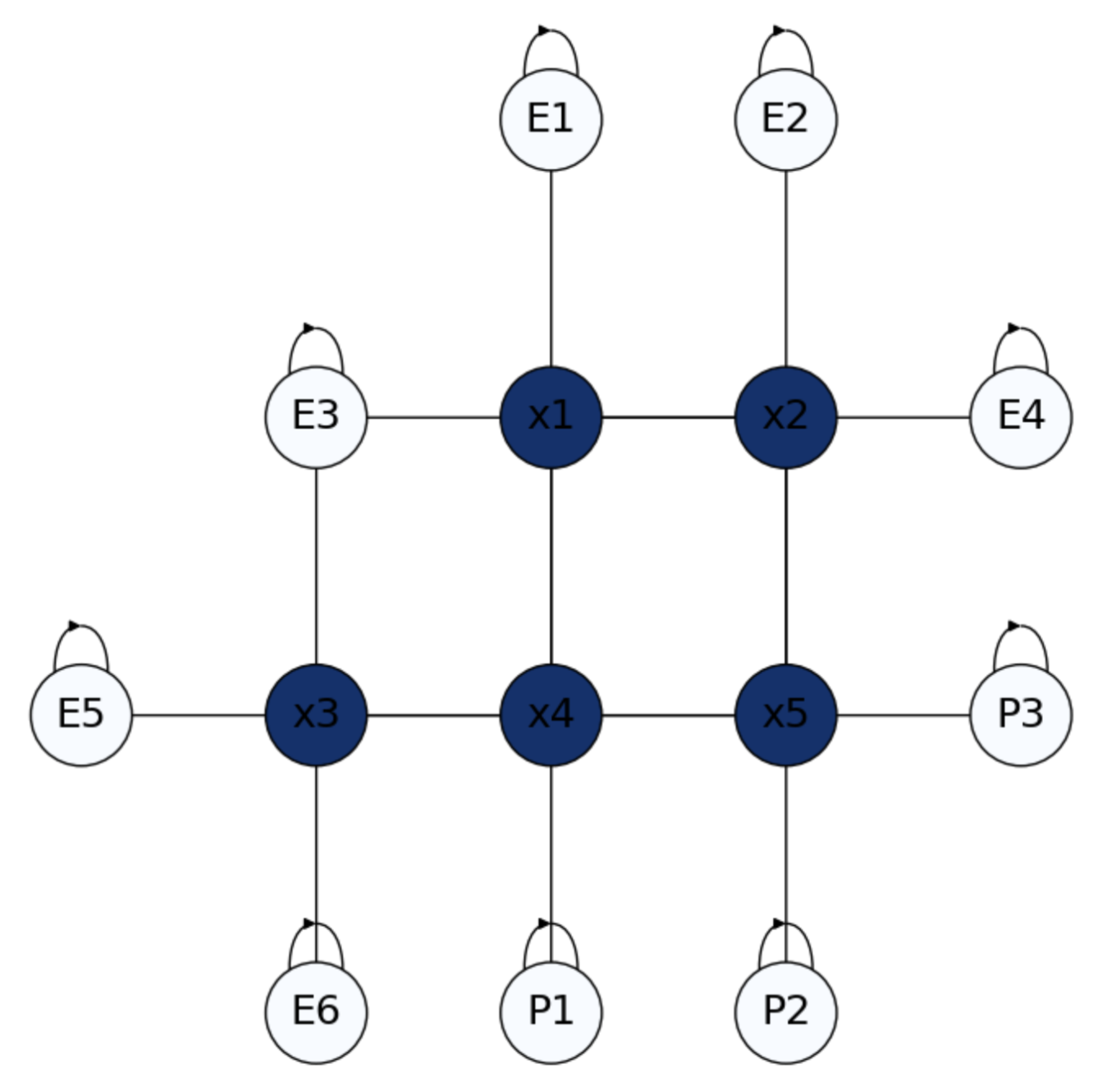
Fig. 4.5 Escape room with Exits \(E_i\) and Policemen \(P_i\) as border nodes.#
Since Exits and Policemen are absorbing states, this is a 2D version of the drunkard’s walk. The game ends when we hit either an Exit, with reward \(1\) or a Policeman, with reward \(0\). Therefore, our problem is to estimate \(p(\text{Exit}|x_i)\) for all \(x_i\).
Imagine that the player starts at node \(x_4\) (close to a policeman and far from an exit). It is reasonable to have \(p(\text{Exit}|x_4)<p(\text{Exit}|x_1)\). Actually if the player “sees” the policeman it will run away, but where? The player does not know the position of the exits and the other policemen in advance. Such info will be propagated to him from the so called border nodes: police-nodes will “send” a reward of \(0\) whereas exits will send a reward of \(1\), though their respective boundary conditions.
Harmonic Principle. Let \(f(i) = p(\text{Exit}|i)\) where \(j\) can be a \(x_j\) a \(E_j\) or a \(P_j\) then, we assume that the probability of an inner node is the average of that of its \(4\) neighbors:
Actually, we have a linear system with \(5\) unknowns \(f(x_1),\ldots,f(x_5)\) and \(5\) equations:
“Harmonicity” ensures that the system has a unique solution and we can solve it very easily if we understand the structure of the system. In the following, even when we use an inverse, we note that actually we do not need to compute it by hand in the exercises but to approximate the solution iteratively.
Transition Matrix. Let \(P\) be a \(n\times n\) matrix, where \(n=|V|\) is the number of nodes of the graph \(G=(V,E)\). Then, the component \(p_{ij}\) is the probability of reaching node \(j\) from node \(i\). For the above escape room, the transition matrix has the following block structure:
where \(n = n_B + n_I\) and \(n_B\) is the number of border (absorbing) nodes and \(n_I\) is the number of interior nodes. Then, we have:
\(\mathbf{I}_{n_B}\) is the identity matrix of dimension \(n_B\). It has the probabilities between border nodes: only self-loops, \(p_{ii}=1\) in the diagonal and \(p_{ij}=0\) for \(j\neq i\).
\(\mathbf{R}_{n_I\times n_B}\) has the probabilities between interior nodes (\(x_1,\ldots,x_5\)) in the rows and border nodes (\(E_1,\ldots,E_6,P_1,P_2, P_3\)) in the cols. In our example, we have \(p_{ij}=1/4\) when \(j\) is a neighbor of \(i\):
\(\mathbf{Q}_{n_I}\) is a square matrix with the probabilities only between interior nodes (\(x_1,\ldots,x_5\)) if any.
An interesting property of \(\mathbf{P}\) is that all rows must sum \(1\) (simple stochastic). Then, note that the sum of probabilities of the same row in \(\mathbf{R}\) and \(\mathbf{Q}\) is actually \(1\) for each row.
What is relation between the two above matrices?The simple stochasticity of \(\mathbf{P}\) gives a precise idea of how to link \(\mathbf{R}\) and \(\mathbf{Q}\) through a linear system.
From one side, we have that \(\mathbf{I}_{n_I}-\mathbf{Q}\) (identity matrix of size \(n_I\) minus \(\mathbf{R}\)) encodes, by adding each row, the probabilities of “escaping towards any absortion node”. For instance, the probability of “escaping” from \(x_2\) towards any of the absortion nodes is \(-\frac{1}{4} + 1 - \frac{1}{4} = \frac{2}{4} = \frac{1}{2}\):
Let \(f = [f_B\; f_D]^T\) be the conditional probabilities \(f(i) = p(\text{Exit}|i)\) where some of them are known (\(f_B=[1\;1\;1\;1\;1\;1\;0\;0\;0]\)) and some others must be estimated (\(f_D\)). With a little abuse of notation, let us denote \(f(x_i)\) as \(x_i\). Then, we have \(f_D = [x_1\;x_2\;x_3\;x_4\;x_5]\).
Then, from the other side, the matrix product \(\mathbf{R}f_B\) encodes the probabilities of going from each interior node to any border one:
As a result, we have the linear system:
The corresponding system in the example is:
Iterative solution. This system, which is equivalent to the one given by the harmonic constrain, is well suited for an iterative solution, without the need of computing the inverse \((\mathbf{I}_{n_I}-\mathbf{Q})^{-1}\).
In this regard, the convergence requirements of the well-known Jacobi Algorithm meet: basically the \(\mathbf{A}\) is diagonally dominant (its entries are greater in absolute value that those the off-diagonal ones). This algorithm obeys the following recurrence relation:
where:
\(\mathbf{D}^{-1}\) is the inverse of \(diag(\mathbf{A})\). In our case it is \(\mathbf{I}_{n_I}\).
\(\mathbf{U}\) and \(\mathbf{L}\) are, respectively, the upper-triangular and lower-triangular sub-matrices of \(\mathbf{A}\) (diagonal not included, i.e. zeroed).
Basically, in this problem, the Jacobi algorithm is extremelly simple:
Thus, setting \(\mathbf{x}_0 = [1\;1\;1\;1\;1]^T\) we have:
which is a good approximation of the exact solution:
As we can see in Fig. 4.6, nodes closer to the Policemen have less probability of success. Maybe the most illustrative example is \(x_4\approx 0.5\), halfway bettween escape and capture!
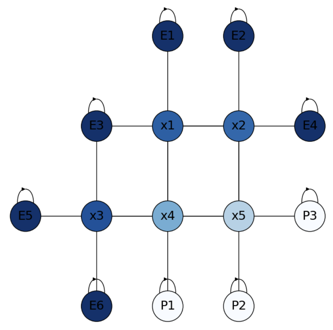
Fig. 4.6 Solution to the Escape Room.#
Obviously, if \(x_i = p(\text{Exit}|i)\), then \(1 - x_i = p(\text{Policemen}|i)\).
Advantages of computing the inverse. The inverse \((\mathbf{I}_{n_I}-\mathbf{Q})^{-1}\) is called the fundamental matrix \(\mathbf{N}\) of the Markov chain (MC). The entries \(N_{ij}\) can be interpreted as the expected number of times that the MC will be in state \(j\) before absortion when it is in state \(i\).
In our example, we have:
Actually, the product \(\mathbf{t}=\mathbf{N}\mathbf{1}\) (column vector of all ones) gives the expected number of steps before absorption for each starting state. Namely
Monte Carlo solution. What if instead of solving a linear system we launch random walks (RWs) from the interior states \(x_1,\ldots, x_5\)? We proceed as follows:
For each \(x_i\) launch \(n\) walks of length \(l\) from each \(x_i\).
The proportion of walks launched from \(x_i\) reach an Exit state is an approximation of \(p(i)=p(\text{Exit}|i)\).
How many walks \(n\) do we need to get a good approximation of \(p\)?
In Binomial terms, \(p(i)\) can be seen as the “probability of success” and we known that when \(n\rightarrow\infty\) we have a normal distribution of mean \(\mu = np\) and standard deviation \(\sigma = \sqrt{npq}\).
Imagine now that the want to ensure that the probability of success is \(.95\).
i.e. \(Z\) is a standarized variable. Due to the symmetry of the normal distribution, the above equation means that the probabilities of the tails satisfy \(p(-a\le Z)=p(Z\ge a)=(1-0.95)/2 = 0.025\). Quering the Standard Normal Cumulative Probability Table we have that \(a = 1.9\approx 2\). Then:
Normizing both the numerator and the denominator by \(n\) we have
leading to
Since \(\sqrt{pq}<1/2\) we have
This means that if we want to ensure that the deviation between the mean \(p(i)\) and the probability of success satisfies
with probability \(0.95\), we need \(n=10,000\) walks for such a small upper bound! Actually the Monte Carlo solution obtained by launching \(10,000\) walks from each interior node is
where the length of each walk is quite flexible (\(l=20\) in this case), since absortion states are pretty close.
Monte Carlo Markov Chains (MCMCs) are very inefficent here but sometimes become an effective search strategy when they are enpowered by data.
Exercise. What if we have negative rewards? In the small problem in Fig. 4.7 we have negative absorbing states \(n_1,\ldots,n_5\) labeled as \(-1\) and positive absorbing states \(p_1\) and \(p_2\) set to \(+1\). In this case, we have only three interior states \(x_1\), \(x_2\) and \(x_3\). What are their probabilities?
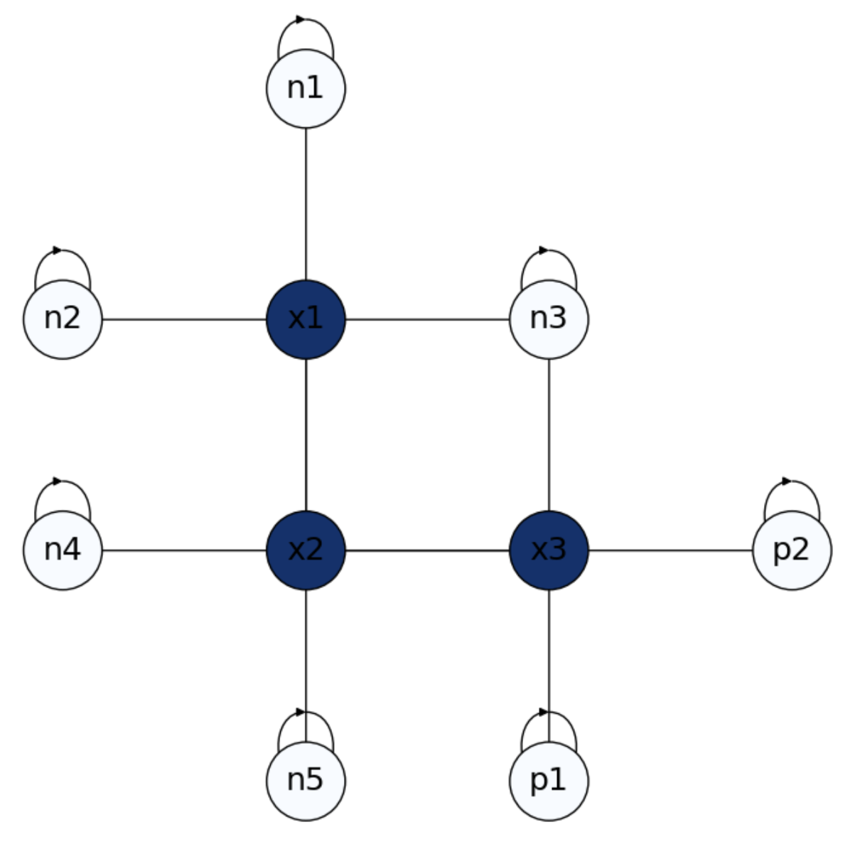
Fig. 4.7 Small Escape Room with positive and negative rewards.#
Let us formulate the matrices \(\mathbf{Q}\) and \(\mathbf{R}\). From \(n_B = 5 + 2 = 7\) and \(n_I = 3\), we have
\(
\mathbf{Q}_{3} =
\begin{bmatrix}
0 & \frac{1}{4} & 0\\
\frac{1}{4} & 0 & \frac{1}{4}\\
0 & \frac{1}{4} & 0\\
\end{bmatrix}
\)
\(
\mathbf{R}_{3\times 7} =
\begin{bmatrix}
\frac{1}{4} & \frac{1}{4} & \frac{1}{4} & 0 & 0 & 0 & 0\\
0 & 0 & 0 & \frac{1}{4} & \frac{1}{4} & 0 & 0\\
0 & 0 & \frac{1}{4} & 0 & 0 & \frac{1}{4} & \frac{1}{4}\\
\end{bmatrix}
\)
Then, from \(f_B = [-1\;-1\;-1\;-1\;-1\;+1\;+1]^T\) and \(f_D = [x_1\;x_2\;x_3]^T\) we set the system
\(
\underbrace{(\mathbf{I}_{3}-\mathbf{Q})}_{\mathbf{A}}\underbrace{f_D}_{\mathbf{x}} = \underbrace{\mathbf{R}f_B}_{\mathbf{b}}\;.
\)
as follows
\(
\begin{bmatrix}
1 & -\frac{1}{4} & 0\\
-\frac{1}{4} & 1 & -\frac{1}{4}\\
0 & -\frac{1}{4} & 1\\
\end{bmatrix}
\begin{bmatrix}
x_1\\
x_2\\
x_3\\
\end{bmatrix} =
\begin{bmatrix}
\frac{1}{4} & \frac{1}{4} & \frac{1}{4} & 0 & 0 & 0 & 0\\
0 & 0 & 0 & \frac{1}{4} & \frac{1}{4} & 0 & 0\\
0 & 0 & \frac{1}{4} & 0 & 0 & \frac{1}{4} & \frac{1}{4}\\
\end{bmatrix}
\begin{bmatrix}
-1\\
-1\\
-1\\
-1\\
-1\\
+1\\
+1\\
\end{bmatrix}
\)
i.e.
\(
\begin{bmatrix}
1 & -\frac{1}{4} & 0\\
-\frac{1}{4} & 1 & -\frac{1}{4}\\
0 & -\frac{1}{4} & 1\\
\end{bmatrix}
\begin{bmatrix}
x_1\\
x_2\\
x_3\\
\end{bmatrix} =
\begin{bmatrix}
-\frac{3}{4}\\
-\frac{2}{4}\\
+\frac{1}{4}\\
\end{bmatrix}
\)
Let us now set and solve the iterative system via Jacobi for these problems:
\(
\mathbf{x}^{t+1} = \mathbf{b} - (\mathbf{L} + \mathbf{U})\mathbf{x}^{t}\;.
\)
\(
\begin{bmatrix}
\mathbf{x}_1^{t+1}\\
\mathbf{x}_2^{t+1}\\
\mathbf{x}_3^{t+1}\\
\end{bmatrix} =
\begin{bmatrix}
-\frac{3}{4}\\
-\frac{2}{4}\\
+\frac{1}{4}\\
\end{bmatrix}-
\begin{bmatrix}
0 & -\frac{1}{4} & 0\\
-\frac{1}{4} & 0 & -\frac{1}{4}\\
0 & -\frac{1}{4} & 0\\
\end{bmatrix}
\begin{bmatrix}
\mathbf{x}_1^{t}\\
\mathbf{x}_2^{t}\\
\mathbf{x}_3^{t}\\
\end{bmatrix}
\)
Thus, setting \(\mathbf{x}_0 = [1\;1\;1]^T\) we have:
\(
\mathbf{x}_1 =
\begin{bmatrix}
-.5\\
0\\
.5\\
\end{bmatrix}\Rightarrow\;
\mathbf{x}_2 =
\begin{bmatrix}
-.75\\
-.5\\
.25\\
\end{bmatrix}\Rightarrow\;
\mathbf{x}_3 =
\begin{bmatrix}
-.875\\
-.625\\
.125\\
\end{bmatrix}\Rightarrow\;
\mathbf{x}_4 =
\begin{bmatrix}
-.90625\\
-.6875\\
.09375\\
\end{bmatrix}\;,
\)
which is a good approximation of the exact solution:
\(
\mathbf{x} =
\begin{bmatrix}
-.92857\\
-.71428\\
.071428\\
\end{bmatrix}\;.
\)
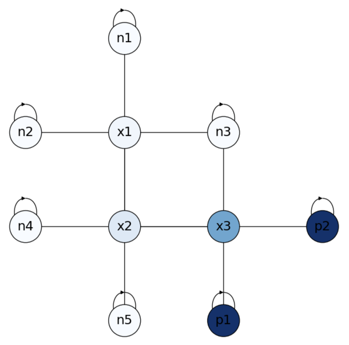
Fig. 4.8 Solution to Small Escape Room with positive and negative rewards.#
As we can see in Fig. 4.8, negative states are closer to negative absorbing states, where \(x_3\) is closer to the positive ones. Remind that \(1-x_i\) gives the probabilities wrt positive absorbing states!
Exercise. Let us solve the drunkard’s walk from this perspective. In Fig. 4.9 we have two absorbing states \(0\) (\(\text{Bar}\)) and \(1\) (\(\text{Home}\)) and four interior states \(x_1\), \(x_2\), \(x_3\) and \(x_4\). We know that \(p(\text{Home}|x_i)=\frac{x_i}{m}\) with \(m=5\) in this case. How to prove that using the 2D aproach?
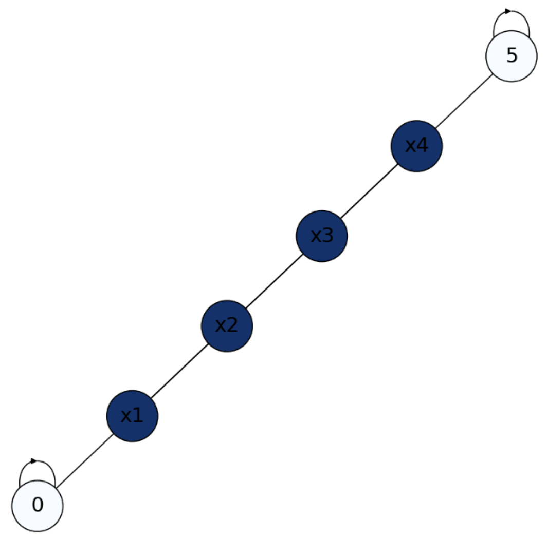
Fig. 4.9 Formulation of the drunkard’s walk with two absorbing states: Bar (0) and Home (5).#
We apply the logic of the Markovian process as follows.
Let us formulate the matrices \(\mathbf{Q}\) (probabilities between interior nodes) and \(\mathbf{R}\) (probabilities between interior and absorbing nodes). From \(n_B = 2\) and \(n_I = 4\), we have
\(
\mathbf{Q}_{4} =
\begin{bmatrix}
0 & \frac{1}{2} & 0 & 0 \\
\frac{1}{2} & 0 & \frac{1}{2} & 0 \\
0 & \frac{1}{2} & 0 & \frac{1}{2} \\
0 & 0 & \frac{1}{2} & 0 \\
\end{bmatrix}
\)
\(
\mathbf{R}_{4\times 2} =
\begin{bmatrix}
\frac{1}{2} & 0 \\
0 & 0 \\
0 & 0 \\
0 & \frac{1}{2}\\
\end{bmatrix}
\)
Then, from \(f_B = [0\;1]^T\) and \(f_D = [x_1\;x_2\;x_3\;x_4]^T\) we set the system
\(
\underbrace{(\mathbf{I}_{4}-\mathbf{Q})}_{\mathbf{A}}\underbrace{f_D}_{\mathbf{x}} = \underbrace{\mathbf{R}f_B}_{\mathbf{b}}\;.
\)
as follows
\(
\begin{bmatrix}
1 & -\frac{1}{2} & 0 & 0\\
-\frac{1}{2} & 1 & -\frac{1}{2} & 0\\
0 & -\frac{1}{2} & 1 & -\frac{1}{2}\\
0 & 0 & -\frac{1}{2} & 1\\
\end{bmatrix}
\begin{bmatrix}
x_1\\
x_2\\
x_3\\
x_4\\
\end{bmatrix} =
\begin{bmatrix}
\frac{1}{2} & 0 \\
0 & 0 \\
0 & 0 \\
0 & \frac{1}{2}\\
\end{bmatrix}
\begin{bmatrix}
0\\
1\\
\end{bmatrix}
\)
i.e.
\(
\begin{bmatrix}
1 & -\frac{1}{2} & 0 & 0\\
-\frac{1}{2} & 1 & -\frac{1}{2} & 0\\
0 & -\frac{1}{2} & 1 & -\frac{1}{2}\\
0 & 0 & -\frac{1}{2} & 1\\
\end{bmatrix}
\begin{bmatrix}
x_1\\
x_2\\
x_3\\
x_4\\
\end{bmatrix} =
\begin{bmatrix}
0\\
0\\
0\\
\frac{1}{2}
\end{bmatrix}
\)
Let us now set and solve the iterative system via Jacobi for this problem:
\(
\mathbf{x}^{t+1} = \mathbf{b} - (\mathbf{L} + \mathbf{U})\mathbf{x}^{t}\;.
\)
\(
\begin{bmatrix}
\mathbf{x}_1^{t+1}\\
\mathbf{x}_2^{t+1}\\
\mathbf{x}_3^{t+1}\\
\mathbf{x}_4^{t+1}\\
\end{bmatrix} =
\begin{bmatrix}
0\\
0\\
0\\
\frac{1}{2}\\
\end{bmatrix}-
\begin{bmatrix}
1 & -\frac{1}{2} & 0 & 0\\
-\frac{1}{2} & 1 & -\frac{1}{2} & 0\\
0 & -\frac{1}{2} & 1 & -\frac{1}{2}\\
0 & 0 & -\frac{1}{2} & 1\\
\end{bmatrix}
\begin{bmatrix}
\mathbf{x}_1^{t}\\
\mathbf{x}_2^{t}\\
\mathbf{x}_3^{t}\\
\mathbf{x}_4^{t}\\
\end{bmatrix}
\)
Thus, setting \(\mathbf{x}_0 = [1\;1\;1\;1]^T\) we have:
\(
\mathbf{x}_1 =
\begin{bmatrix}
.5\\
1\\
1\\
1\\
\end{bmatrix}\Rightarrow\;
\mathbf{x}_2 =
\begin{bmatrix}
.5\\
.75\\
1\\
1\\
\end{bmatrix}\Rightarrow\;
\mathbf{x}_3 =
\begin{bmatrix}
.375\\
.75\\
.875\\
1\\
\end{bmatrix}\Rightarrow\;
\mathbf{x}_4 =
\begin{bmatrix}
.375\\
.625\\
.875\\
.9375\\
\end{bmatrix}\;,
\)
which is a reasonable approximation of the exact solution:
\(
\mathbf{x} =
\begin{bmatrix}
.2\\
.4\\
.6\\
.8\\
\end{bmatrix}\;.
\)
See Fig. 4.10, darker states are closer to \(\text{Home}\). Remind that \(1-x_i\) gives the probabilities wrt the \(\text{Bar}\)!
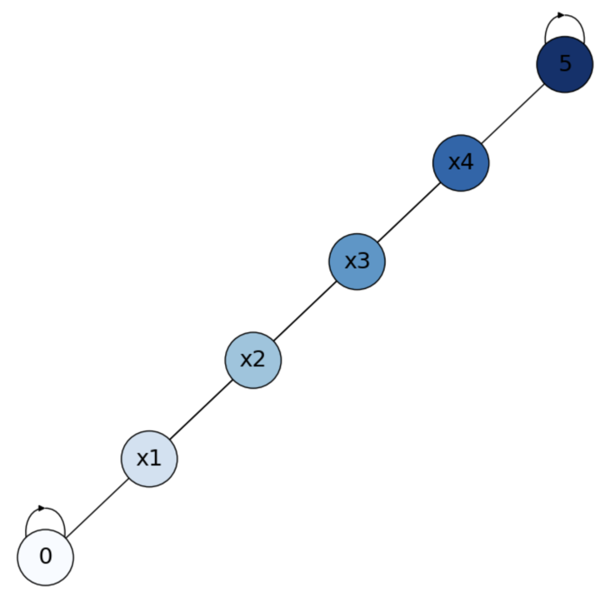
Fig. 4.10 Solution to Small Escape Room with positive and negative rewards.#
4.4. The Cutoff Phenomenon#
4.4.1. Markov chains and equilibrium#
When studying Markov Chains (MCs) we have left intentionally appart one fundamental aspect of them: their long-time behaviors. This includes, of course, their limiting distributions or steady states. The quest for harmonicity, for instance, gives us some search for equilibrium in the linear system. See for instance Fig. 4.8, where the numerical solution to this system ensures that the state of an interior node converges to the average of its neighbors (which may include other interior nodes or border/absorbing ones). Actually, harmonicity implies equilibrium and vice versa as we will show later on, as a first example of Spectral Graph Theory.
4.4.2. Shuffling cards#
For the moment, a rough idea of this concept is to identify equilibrium with complete disorder or randomness. Consider for instance a mini-deck of cards consisting only of the \(n=13\) cards of the \(\heartsuit\) suit. Initially, this deck is ordered according to their increasing face values, i.e. we have
A riffle suffling consists of:
1- Select a cut point \(k\) (approximately at \(1/2\) of the mini-deck) so that we divide the deck into \(2\) packets of similar size: \(1,2,\ldots,k\) and \(k+1,k+2,\ldots,n\). For \(k=6\) we have:
2- Interleave the two subdecks so that the relative positions within each subdeck is preserved and then form a new mini-deck:
A rising sequence is a maximal subset of cards where their successive values are displayed in increasing order. For instance, in the previous interleaving we have two rising sequences: \(A\), \(2\), \(3\), \(4\), \(5\), \(6\) and \(7\), \(8\), \(9\), \(10\), \(J\), \(Q\), \(K\). Actually, these rising sequences come from the first cut, so the rising sequences can be used to reconstruct the original order of the deck.
What happens if we perform another riffle shuffle? Now we select \(k=7\) for cutting and we have:
Before interleaving the cards, we have that each pack has \(2\) rising sequences:
\(A\), \(2\), \(3\) and \(7\), \(8\), \(9\), \(10\) for the left pack.
\(4\), \(5\), \(6\) and \(J\), \(Q\), \(K\) for the right pack.
This means that before mixing the cards we have doubled the number of rising sequences.
Let us interleave the two packs above:
with rising sequences:
\(A\), \(2\), \(3\).
\(4\), \(5\), \(6\).
\(7\), \(8\), \(9\), \(10\).
\(J\), \(Q\), \(K\).
Effectively, each new riffle shuffle tends to double the number of rising sequences until the capacity of the deck is reached. What is such a capacity? Since \(2^{3}<13<2^{4}\), after \(4\) shuffles we will have the mini-deck completely mixed. Why? Because for \(a=4\) riffle shuffles we have \(13\) rising sequences, i.e. the mini-deck in descending order:
If we have \(n\) cards, the maximum number of rising sequences is \(n\), i.e. every card \(c_i\) has a face value higher than \(c_{i+1}\) for \(i=1,2,\ldots,n-1\). Thus for \(n=52\) cards we need \(2^{a}\approx 52\) riffle shuffles, i.e. \(a=6\). Aldous and Diaconis proved that we need \(a=7\) riffle shuffles to ensure complete disorder. In any case we have that \(a\) is \(O(log_2 n)\).
The cutoff phenomenon refers to the fact that when measuring how close we are from complete randomness, most of the time we are very far away. However, at a certain point, we drastically become very close to randomness. Not all Markov chains have this property, but when they have it, that point is called the cutoff point.