6. Ranking and Partitions

6.1. Transition matrix

Given a (undirected) graph \(G=(V,E)\), we consider:

• The adjacency matrix \(\mathbf{A}=[a_{ij}]\in \{0,1\}^{n\times n}\) of dimension \(n\times n\), where \(n=|V|\) is the number of nodes, and

\[\begin{split} a_{ij}= \begin{cases} 1\;\text{if}\; (i,j)\in E \\[2ex] 0\; \text{otherwise}\;. \end{cases} \end{split}\]

• The degree matrix \(\mathbf{D}=[d_i]\) is an \(n\times n\) diagonal matrix where \(d_i = \sum_{j}a_{ij}\) is the degree \(\text{deg}(i)\) of node \(i\).

Then, if the graph has no isolated nodes (none of them has zero degree) the so called transition matrix \(\mathbf{P}=[p_{ij}]\), encoding the Markov chain associated with the nodes of the graph, is given by

\[ \mathbf{P} = \mathbf{D}^{-1}\mathbf{A}\;\;\text{i.e.}\;\; p_{ij} = \frac{a_{ij}}{d_i}\;. \]

It is very interesting to remark the following properties of \(\mathbf{P}\):

• Simply Stochastic (by rows). All the rows \(i=1,2,\ldots, n\) satisfy:

\[ \sum_{j=1}^n p_{ij} = 1\;. \]

i.e. each row \(\mathbf{P}_{i:}\) (associated to a node \(i\)) can be interpreted as a probability distribution.

• Rank deficient. In general, \(\mathbf{P}\) is not invertible, i.e. \(\text{rank}(\mathbf{P})\ll n\), and the higher the rank the more different (and thus informative) are the row probability distributions.

6.1.1. Stationary Distribution

When we studied Markov chains in the context of random walks, we left aside the use of \(\mathbf{P}\) for characterizing the Markov chain in the limit. This means that we can obtain very interesting information about the nodes in \(G=(V,E)\) by analyzing the powers \(\mathbf{P}^k\) for increasing values of \(k=1,2,\ldots,\infty\).

Let us start by understanding the meaning of \(\mathbf{P}\), \(\mathbf{P}^2\), \(\mathbf{P}^3\), etc. Actually \(\mathbf{P}^k_{ij}\) is the probability of reaching node \(j\) from \(i\) in \(k\) steps or hops.

Depending on the graph \(G=(V,E)\) we may need only a small number of powers \(k\). Consider for instance the complete graph or clique graph for \(n\) nodes, dubbed \(K_n\). The complete graph is the denser graph than one can imagine since it has \(n\) nodes and each node has \(n\) links (including self-loops). Therefore, the adjacency matrix of \(K_n\) is:

\[ \mathbf{A} = \mathbf{1}\mathbf{1}^T\;, \]

where \(\mathbf{1}\) is the \(n\times 1\) vector of all ones, i.e. \(\mathbf{A}\) is a matrix of ones.

Well, the degree of each node in \(K_n\) is constant for each node and equal to \(n\). Therefore, the transition matrix is

\[ \mathbf{P} = \frac{1}{n}\mathbf{A},\;\; \text{with}\;\; p_{ij}=\frac{1}{n}\; \forall i,j\;. \]

Then every node \(i\) has the same probability of going to any other \(j\) (including itself) in only one hop. In other words, a node \(i\) does not need to visit first any other node before hitting \(j\). This makes \(\mathbf{P}^2\), \(\mathbf{P}^3\), etc, redundant since

\[ \mathbf{P}^2 = \frac{1}{n}\mathbf{1}\mathbf{1}^T\cdot \frac{1}{n}\mathbf{1}\mathbf{1}^T = \frac{1}{n^2}n\mathbf{1}\mathbf{1}^T = \frac{1}{n}\mathbf{1}\mathbf{1}^T=\mathbf{P}\;. \]

This means that in \(K_n\) (as well as in hyper-dense graphs), all the nodes have the same structural role. Note that in these case we have \(\text{rank}(\mathbf{P})=1\).

However, in more general graphs we can identify or rank the structural role of each node by analyzing \(\mathbf{P}^k\) for increasing values of \(k\).

Consider, for instance a Stochastic Block Model (SBM) graph of \(n=20\) nodes with intra-class probaility \(p=0.75\) and inter-class probability \(q=0.05\) (see Fig. 6.1).

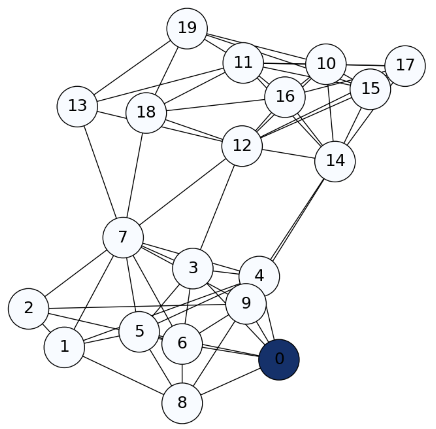
Fig. 6.1 SBM graph. Diffusion from \(i=1\) (\(0\) in the picture) at \(\mathbf{f}^0\).

Imagine that we inject information into node \(i=0\) and see how such information is diffused through the graph. We do that by setting a row-probability vector \(\mathbf{f}\) as follows:

\[ \mathbf{f}^0 = [1\; 0\;\ldots\; 0]\;. \]

Then, decomposing \(\mathbf{P}=[\mathbf{P}_{:1}\;\mathbf{P}_{:2}\;\ldots\; \mathbf{P}_{:n}]\) in terms of its columns \(\mathbf{P}_{:j}\) we have

\[ \mathbf{f}^1 = \mathbf{f}^0\mathbf{P} = [\mathbf{f}^0\mathbf{P}_{:1}\;\mathbf{f}^0\mathbf{P}_{:2}\;\ldots\;\mathbf{f}^0\mathbf{P}_{:n}] \]

where, starting at a general node \(i\) leads to

\[ \mathbf{f}^1_i = \sum_{j=1}^n\mathbf{f}^0_ip_{ij} = \sum_{j\in {\cal N}_i}^n\mathbf{f}^0_ip_{ij}\;. \]

In particular, for \(i=1\) we have a row vector \(\mathbf{f}^1\) with \(\mathbf{f}^1_i=p_{1j}\), i.e. we may reach any of the other nodes \(j\) with probability \(p_{1j}\). As we see in Fig. 6.2, in a first diffusion step, we only reach the nodes in the neigborhood of node \(i=1\).

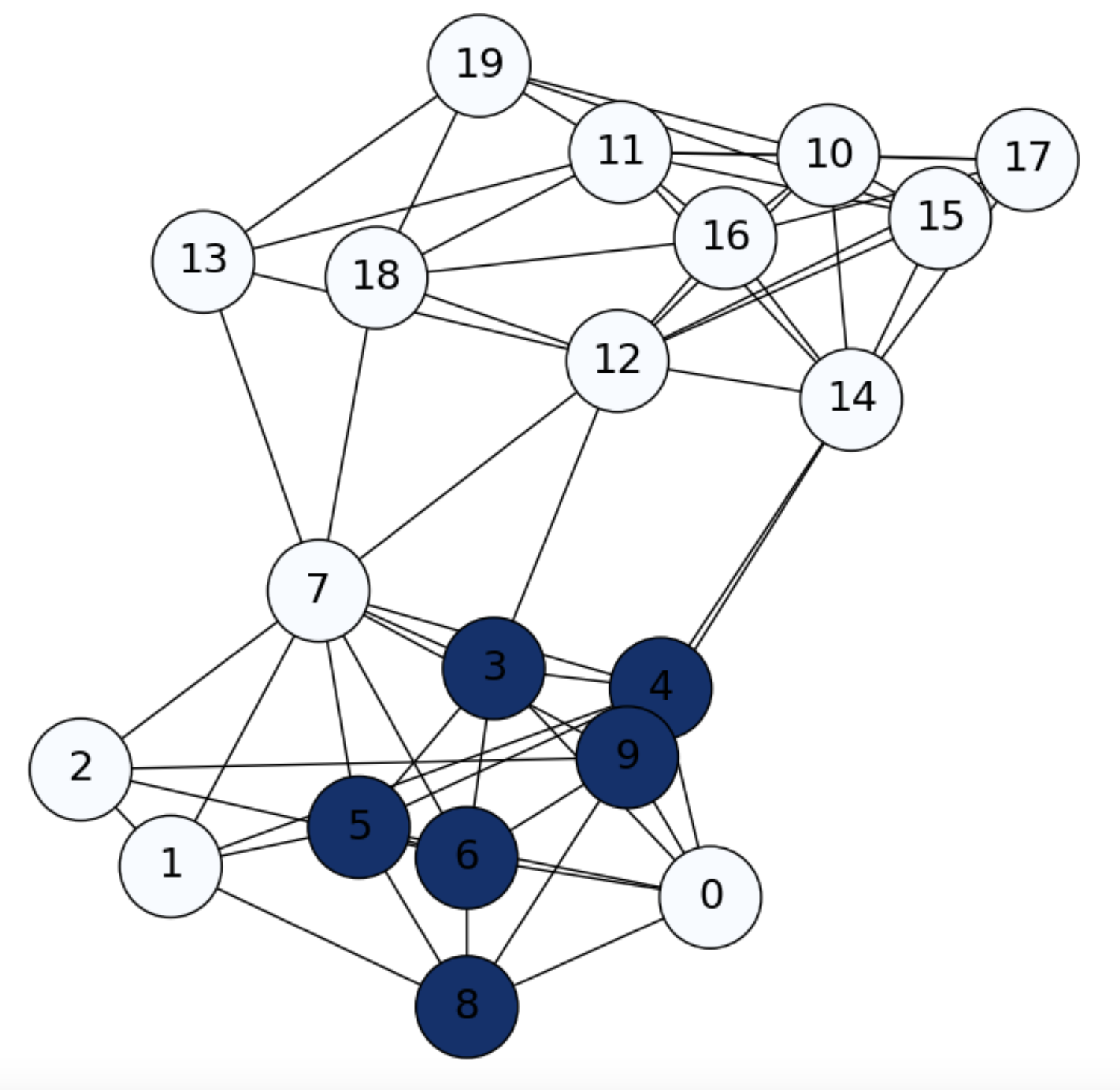
Fig. 6.2 SBM graph. Diffusion from \(i=1\) (\(0\) in the picture) at \(\mathbf{f}^1\).

Let us iterate again:

\[ \mathbf{f}^2_i = \sum_{j=1}^n\mathbf{f}^1_ip_{ij} = \sum_{j\in {\cal N}_i}^n\mathbf{f}^1_ip_{ij}\;. \]

Since,

\[ \mathbf{f}^1\mathbf{P}=(\mathbf{f}^0\mathbf{P})\mathbf{P} = \mathbf{f}^0\mathbf{P}^2\;, \]

we may reach the second-order neighbors of node \(i\), i.e. the nodes that are two-hops away from \(i\), in particular some nodes of another community, as we see in Fig. 6.3.

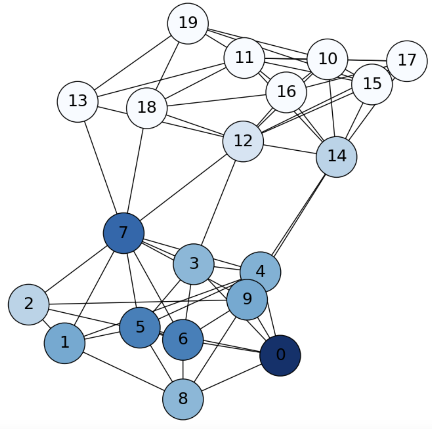
Fig. 6.3 SBM graph. Diffusion from \(i=1\) (\(0\) in the picture) at \(\mathbf{f}^2\).

Iterating again we state that we are more probable to be in the community of \(i=1\), but we may jump to another community (see Fig. 6.4):

\[ \mathbf{f}^3_i = \sum_{j=1}^n\mathbf{f}^2_i p_{ij} = \sum_{j\in {\cal N}_i}^n\mathbf{f}^2_ip_{ij}\;. \]

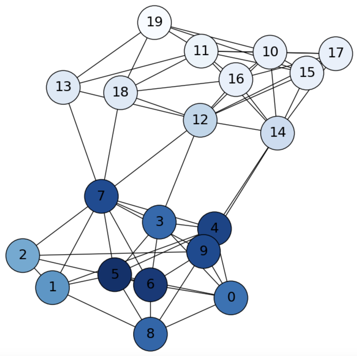
Fig. 6.4 SBM graph. Diffusion from \(i=1\) (\(0\) in the picture) at \(\mathbf{f}^3\).

Then, two interesting question arise:

1. For what \(t\) are the probabilities in \(\mathbf{f}^{t}\) stabilized?

2. Is that stabilized probability the same for all choices of starting node.?

Stationary distribution. Under certain conditions (see below) the answer to both questions is Yes.

For \(t\rightarrow\infty\) we have that if we reach a given row-distribution \(\pi\), the resulting \(\pi\mathbf{P}\) is exactly \(\pi\), where

\[ \pi = \pi\mathbf{P}\;\;\text{and}\;\;\pi_i = \frac{d_i}{\text{vol}(G)}\;, \]

and \(\text{vol}(G)=\sum_{i=1}^n d_i\) is the volume of the graph (\(\text{vol}(G)=2|E|\) for undirected graphs). In other words, \(\pi\) is a fixed point known as the stationary distribution of \(\mathbf{P}\). Actually it is very straight to prove that

\[ d_i = \sum_{j\in {\cal N}_i}d_ip_{ij} = \sum_{j\in {\cal N}_i}\frac{d_i}{d_i} = \sum_{j\in {\cal N}_i}1 = d_i\;. \]

Then, the stationary distribution \(\pi\) is the result of normalizind the degree distribution by the volume.

In our example, we show the stationary distribution for our SBM in Fig. 6.5.

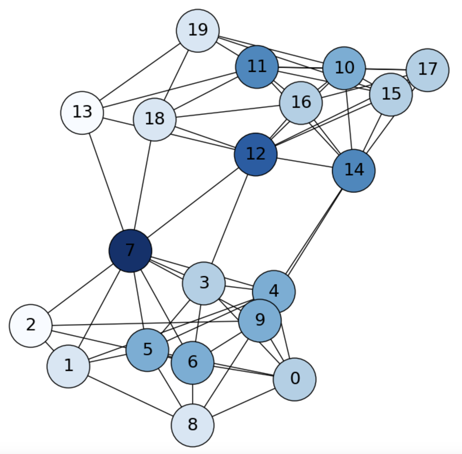
Fig. 6.5 SBM graph. Stationary distribution \(\pi\).

In other words, reaching the stationary distribution in \(t\) hops means that from any discrete time \(t+\Delta t\), the probability of being at any node \(i\) is only dependent on its degree \(d_i\).

To clarify this point, note that we have that

\[ \lim_{t\rightarrow\infty}\mathbf{P}^t = \Pi\; \]

and \(\Pi\) is a matrix where each row is a copy of the stationary distribution \(\pi\). Look for instance at the row \(i\):

\[ \Pi_{i:} = \pi = [\frac{d_1}{\text{vol}(G)}\; \frac{d_2}{\text{vol}(G)}\;\ldots\; \frac{d_n}{\text{vol}(G)}\;]\;, \]

i.e. the probability of going from \(i\) to any other node \(j\) is proportional to \(d_j\), indendendently of whether \(j\) is a neighbor of \(i\) or not!

Consider now the complete graph \(K_n\), where each node can visit any other (including itself) with probability \(\frac{1}{n} = \frac{n}{n^2}=\frac{d_i}{\sum_{i}d_i}\). In other words, a complete graph is a graph that has reached its stationary distribution at time \(t=0\).

Formal conditions. The stationary distribution is unique if:

1. The Markov chain is irreducible (all the states \(i\) and \(j\) are mutually reachable). For undirected graph it is enough that the graph is connected. For digraphs we must ensure that exists a directed path between any pair of nodes with is more difficult to achieve in realistic networks.

2. The Markov chain is aperiodic. For satisfying this consition, we need that if there exists a positive integer \(k\) s.t. all the entries in \(\mathbf{P}^k\) are greater than zero. A less strict condition is to have at least a node with a self loop.

6.1.2. The Spectral Interpretation: PageRank

The stationary distribution \(\pi\), reshaped as a \(n\times 1\) vector can be considered as a left eigenvector of the transition matrix for the eigenvalue \(\lambda=1\) since

\[ \phi^T\mathbf{P} = \lambda\phi^T\;\;\text{leads to}\; \pi^T\mathbf{P} = 1\cdot\pi^T\;. \]

Similarly, the right eigenvectors and eigenvalues (typically we calculate these ones) are defined as:

\[ \mathbf{P}\psi = \lambda\psi\;\;\text{leads to}\; \mathbf{P}\psi = 1\cdot\psi\;. \]

Looking at the above equations, in the next topic we will prove that \(\psi = \mathbf{D}^{1/2}\mathbf{1}\) is the right eigenvector of the transition matrix \(\mathbf{P}\).

The meaning of \(\psi = \mathbf{D}^{1/2}\mathbf{1}\) is that

\[ \psi_i = \sqrt{d_i}\; \]

is related to \(\pi_i = \frac{d_i}{\text{vol}(G)}\), in terms that it is a monotonic function of \(d_i\). Both \(\pi\) and \(\psi\) rank the importance of a node in the graph in terms of its degree.

As we will see below, computing the right eigenvector is very interesting in practical settings, since it can be approximated even in networks/graphs not satisfying the formal conditions of irreducibility and aperiodicity!

Perron-Frobenius Theorem. If \(\mathbf{M}\) is a positive, column stochastic matrix, then:

1. \(\lambda=1\) is an eigenvalue of multiplicity one (unique).

2. \(\lambda=1\) is the largest eigenvalue: all the other eigenvalues have absolute value smaller than 1.

3. The eigenvectors corresponding to the eigenvalue \(\lambda=1\) have either only positive entries or only negative entries.

4. In particular, for the eigenvalue \(\lambda=1\) there exists a unique eigenvector with the sum of its entries equal to 1 (a probability distribution).

Then \(\mathbf{M}=\mathbf{P}^T\) satisfies this theorem. As in general every square matrix has the same eigenvalues as its transpose, we will approximate the left eigenvector of \(\mathbf{P}\) by computing

\[ \mathbf{P}^T\phi = (\phi^T\mathbf{P})^T = 1\cdot \phi\;. \]

and in practice we may approximate the eigenvector \(\phi\) associated to \(\lambda=1\) in an iterative way. To that end we use the Power Method. As we show in Power, all we do is to:

Algorithm 6.1 (Power Method)

Inputs Given an \(n\times n\) matrix \(\mathbf{M}\) and \(\mathbf{x}=\frac{1}{n}\mathbf{1}\)

Output Compute an approximation of the main eigenvector \(\phi\)

1. for each of the \(k\) iterations:

   1. \(\mathbf{x}\;\leftarrow \mathbf{M}\mathbf{x}\)

   2. Normalize: \(\mathbf{x} \;\leftarrow \frac{\mathbf{x}}{||\mathbf{x}||}\)

2. return \(\mathbf{x}\)

1. Initialize \(\mathbf{x}_i = \frac{1}{n}\) (completely random estimation of the eigenvector).

2. For \(M=\mathbf{P}^T\) compute \(\mathbf{M}\mathbf{x}, \mathbf{M}^2\mathbf{x},\ldots, \mathbf{M}^k\mathbf{x}\).

3. Between one power and the next, normalize the current eigenvector \(\mathbf{x}\).

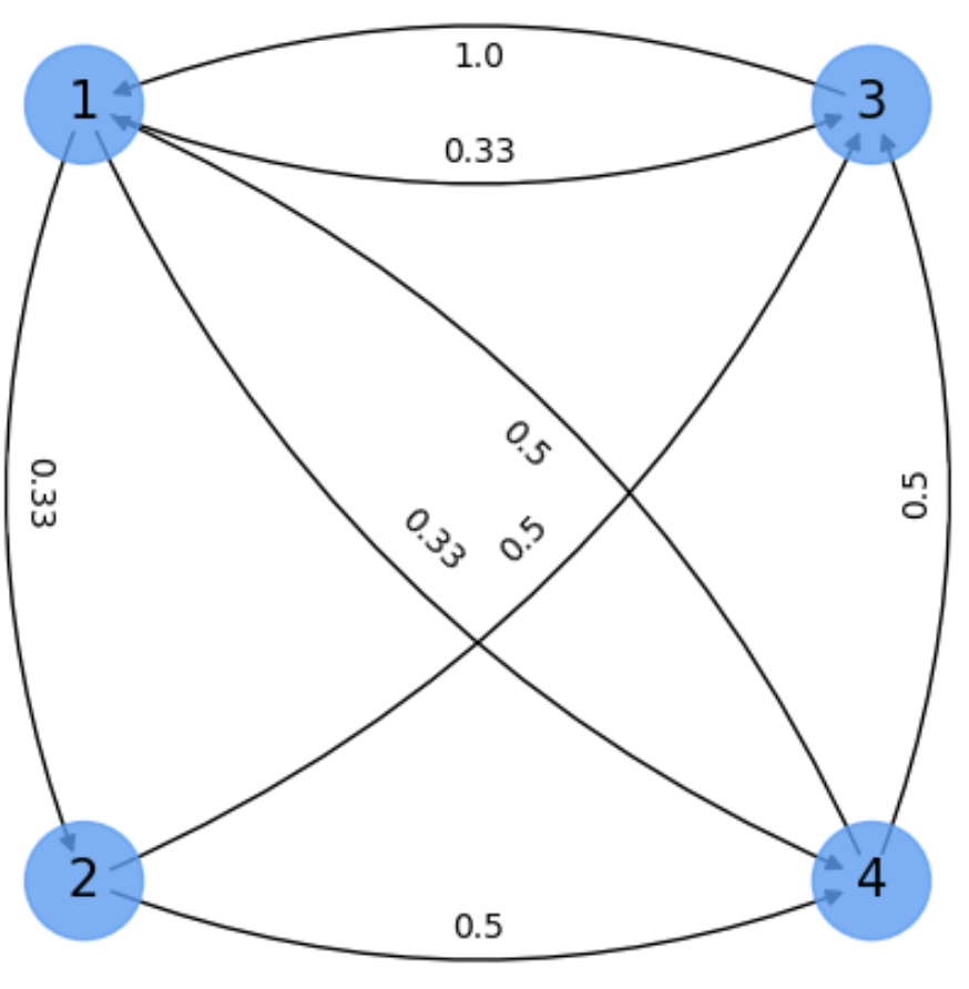
Fig. 6.6 Small digraph for computing the main eigenvector.

Exercise. Our digraph Fig. 6.6 is not aperiodic. This problem is not so hard as not being irreducible. In particular all the nodes are mutually reachable and this allows us to get a nice approximation.

\( \mathbf{x}_0=\frac{1}{n}\mathbf{1} = \begin{bmatrix} \frac{1}{4}\\ \frac{1}{4}\\ \frac{1}{4}\\ \frac{1}{4}\\ \end{bmatrix}\;\; \mathbf{x}_1 = \mathbf{P^T}\mathbf{x}_0 = \begin{bmatrix} 0 & 0 & 1 & \frac{1}{2}\\ \frac{1}{3} & 0 & 0 & 0 \\ \frac{1}{3} & \frac{1}{2} & 0 & \frac{1}{2}\\ \frac{1}{3} & \frac{1}{2} & 0 & 0 \\ \end{bmatrix} \begin{bmatrix} \frac{1}{4}\\ \frac{1}{4}\\ \frac{1}{4}\\ \frac{1}{4}\\ \end{bmatrix} = \begin{bmatrix} 0.375\\ 0.083\\ 0.333\\ 0.208\\ \end{bmatrix} \)

\( \mathbf{x}_1=\frac{\mathbf{x}_1}{||\mathbf{x}_1||} = \begin{bmatrix} 0.682\\ 0.151\\ 0.606\\ 0.379\\ \end{bmatrix}\;\; \mathbf{x}_1 = \mathbf{P^T}\mathbf{x}_0 = \begin{bmatrix} 0 & 0 & 1 & \frac{1}{2}\\ \frac{1}{3} & 0 & 0 & 0 \\ \frac{1}{3} & \frac{1}{2} & 0 & \frac{1}{2}\\ \frac{1}{3} & \frac{1}{2} & 0 & 0 \\ \end{bmatrix} \begin{bmatrix} 0.682\\ 0.151\\ 0.606\\ 0.379\\ \end{bmatrix} = \begin{bmatrix} 0.796\\ 0.227\\ 0.492\\ 0.303\\ \end{bmatrix} \)

\( \mathbf{x}_2=\frac{\mathbf{x}_2}{||\mathbf{x}_2||} = \begin{bmatrix} 0.788\\ 0.225\\ 0.487\\ 0.300\\ \end{bmatrix}\;\; \mathbf{x}_2 = \mathbf{P^T}\mathbf{x}_1 = \begin{bmatrix} 0 & 0 & 1 & \frac{1}{2}\\ \frac{1}{3} & 0 & 0 & 0 \\ \frac{1}{3} & \frac{1}{2} & 0 & \frac{1}{2}\\ \frac{1}{3} & \frac{1}{2} & 0 & 0 \\ \end{bmatrix} \begin{bmatrix} 0.788\\ 0.225\\ 0.487\\ 0.300\\ \end{bmatrix} = \begin{bmatrix} 0.637\\ 0.262\\ 0.525\\ 0.375\\ \end{bmatrix} \)

at iteration \(10\) we wil have \( \mathbf{x}_{9}=\frac{\mathbf{x}_{9}}{||\mathbf{x}_{9}||} = \begin{bmatrix} 0.720\\ 0.240\\ 0.541\\ 0.361\\ \end{bmatrix}\;\; \mathbf{x}_{10} = \mathbf{P^T}\mathbf{x}_9 = \begin{bmatrix} 0 & 0 & 1 & \frac{1}{2}\\ \frac{1}{3} & 0 & 0 & 0 \\ \frac{1}{3} & \frac{1}{2} & 0 & \frac{1}{2}\\ \frac{1}{3} & \frac{1}{2} & 0 & 0 \\ \end{bmatrix} \begin{bmatrix} 0.720\\ 0.240\\ 0.541\\ 0.361\\ \end{bmatrix} = \begin{bmatrix} 0.722\\ 0.240\\ 0.540\\ 0.360\\ \end{bmatrix}\;. \)

Therefore, the most important node is node \(1\), followed by nodes \(3\), \(4\) and \(2\). Note that this result is quite different from the stationary distribution estimated in terms of out degrees:

\( \pi = \frac{\mathbf{D}_{out}\mathbf{1}}{\text{vol}(G)} = \begin{bmatrix} 0.375\\ 0.25\\ 0.125\\ 0.25\\ \end{bmatrix}\;. \)

And also different from the theoretical right eigenvector:


\( \psi = \sqrt{\mathbf{D}_{out}}\mathbf{1} = \begin{bmatrix} 1.732\\ 1.414\\ 1.000\\ 1.414\\ \end{bmatrix}\;. \)

Although in both cases, the top ranked node is correctly detected.

The Google Pagerank. One of the most representative applications of the power method is to find the rankings of the web pages in the Internet. The higher the values (in absolute value) of the components of the resulting main eigenvector \(\mathbf{x}\) the more important the page.

However, Internet (which can be considered a gigantic graph whose nodes are the web pages), does not necessarily meet the formal conditions needed for the unicity or convergence of \(\mathbf{x}\).

For instance, in Fig. 6.7 we summarize the main practical problems arising in realistic networks:

• Sources: nodes only with out degree, such as node \(2\) which is only linked to \(3\) and \(4\).

• Sinks: node with zero out degree, such as node \(3\).

In addition we may have isolated nodes or graphs fragmented in many connected components.

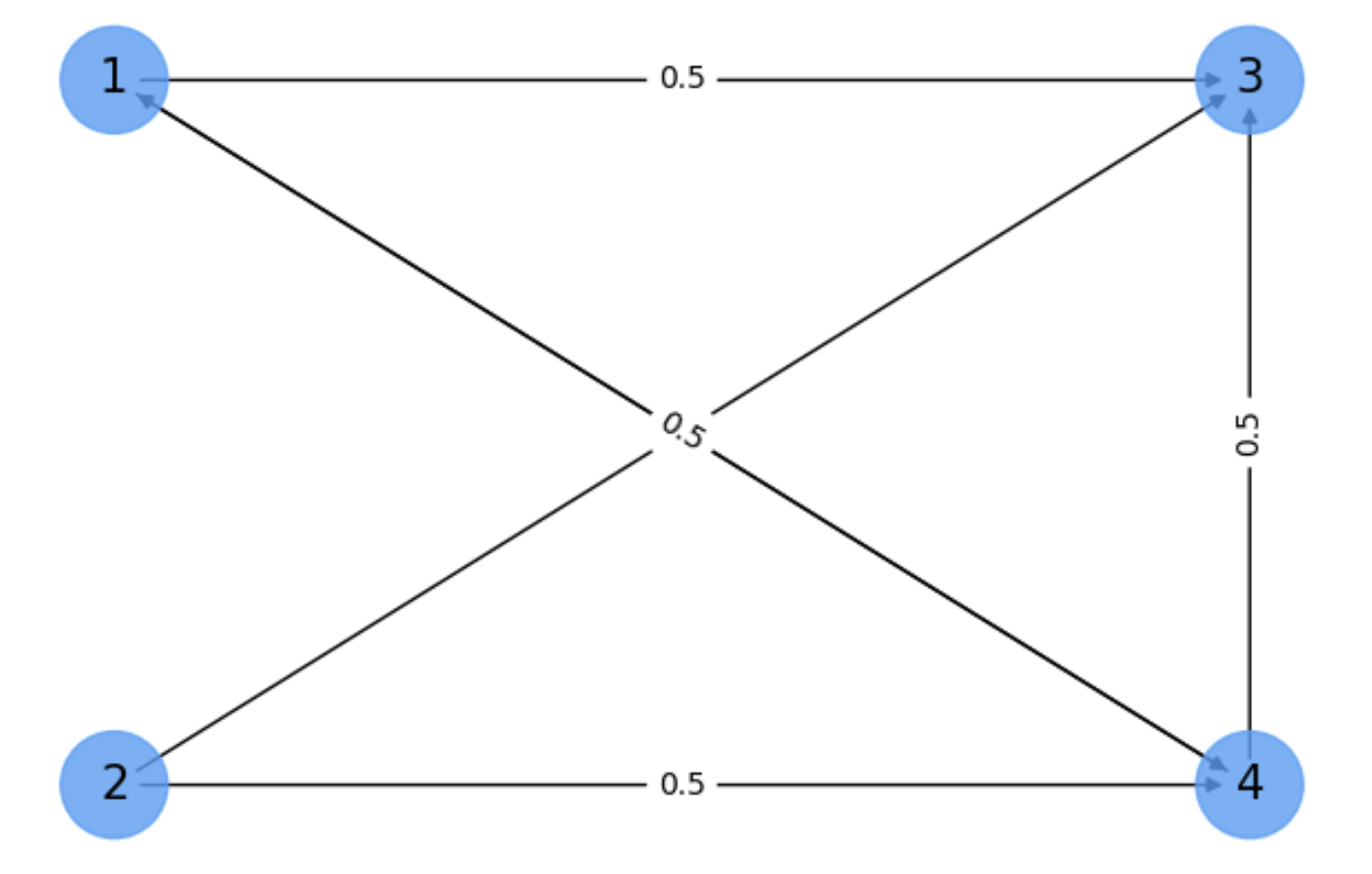
Fig. 6.7 Pagerank. Need of the Google matrix.

The solution to these problems found by Page and Bruin when designing a model for the Google Internet surfer, was to complement the transition matrix (actually its transpose), with a complete graph so that with certain probability \(1-\alpha\) (typically \(1-\alpha=0.85\)) we follow the transition matrix, but with a small probability \(\alpha=0.15\) (dubbed the teleporting probability) we jump randomly to any other node or stay at the same mode (self-loop). Therefore, the so called Google matrix:

\[ \mathbf{G} = (1-\alpha)\cdot\mathbf{P}^T + \alpha\cdot\frac{1}{n}\mathbf{1}^T\mathbf{1}\; \]

Therefore, the Google matrix consists of adding virtual edges between any pair of nodes (including self-loops). This makes the resulting Markov chain irreducible with facilitates information flow. In this regard, finding what is the probability that a surfer ends up clicking a given page is done via the Power method.

Exercise. We repeat the previous exercise by using the Google matrix for the digraph in Fig. 6.7.

\( \mathbf{x}_0=\frac{1}{n}\mathbf{1} = \begin{bmatrix} \frac{1}{4}\\ \frac{1}{4}\\ \frac{1}{4}\\ \frac{1}{4}\\ \end{bmatrix}\;\; \mathbf{x}_1 = \mathbf{G}\mathbf{x}_0 = \begin{bmatrix} \alpha\frac{1}{4} & \alpha\frac{1}{4} & \alpha\frac{1}{4} & (1-\alpha)\frac{1}{2}\\ \alpha\frac{1}{4} & \alpha\frac{1}{4} & \alpha\frac{1}{4} & \alpha\frac{1}{4} \\ (1-\alpha)\frac{1}{2} & (1-\alpha)\frac{1}{2} & \alpha\frac{1}{4} & (1-\alpha)\frac{1}{2}\\ (1-\alpha)\frac{1}{2} & (1-\alpha)\frac{1}{2} & \alpha\frac{1}{4} & \alpha\frac{1}{4} \\ \end{bmatrix} \begin{bmatrix} \frac{1}{4}\\ \frac{1}{4}\\ \frac{1}{4}\\ \frac{1}{4}\\ \end{bmatrix} = \begin{bmatrix} \alpha\frac{1}{16} + \frac{2}{16}\\ \alpha\frac{4}{16}\\ \frac{6}{16}-\alpha\frac{5}{16}\\ \frac{4}{16}-\alpha\frac{2}{16}\\ \end{bmatrix} \)

\( \mathbf{x}_1=\frac{\mathbf{x}_1}{||\mathbf{x}_1||} = \begin{bmatrix} 0.312\\ 0.081\\ 0.774\\ 0.543\\ \end{bmatrix}\;\; \mathbf{x}_2 = \mathbf{G}\mathbf{x}_1 = \begin{bmatrix} \alpha\frac{1}{4} & \alpha\frac{1}{4} & \alpha\frac{1}{4} & (1-\alpha)\frac{1}{2}\\ \alpha\frac{1}{4} & \alpha\frac{1}{4} & \alpha\frac{1}{4} & \alpha\frac{1}{4} \\ (1-\alpha)\frac{1}{2} & (1-\alpha)\frac{1}{2} & \alpha\frac{1}{4} & (1-\alpha)\frac{1}{2}\\ (1-\alpha)\frac{1}{2} & (1-\alpha)\frac{1}{2} & \alpha\frac{1}{4} & \alpha\frac{1}{4} \\ \end{bmatrix} \begin{bmatrix} 0.312\\ 0.081\\ 0.774\\ 0.543\\ \end{bmatrix} = \begin{bmatrix} 0.295\\ 0.064\\ 0.462\\ 0.231\\ \end{bmatrix} \)

at iteration \(10\) we wil have

\( \mathbf{x}_9=\frac{\mathbf{x}_9}{||\mathbf{x}_9||} = \begin{bmatrix} 0.264\\ 0.066\\ 0.484\\ 0.286\\ \end{bmatrix}\;\; \mathbf{x}_{10} = \mathbf{G}\mathbf{x}_9 = \begin{bmatrix} \alpha\frac{1}{4} & \alpha\frac{1}{4} & \alpha\frac{1}{4} & (1-\alpha)\frac{1}{2}\\ \alpha\frac{1}{4} & \alpha\frac{1}{4} & \alpha\frac{1}{4} & \alpha\frac{1}{4} \\ (1-\alpha)\frac{1}{2} & (1-\alpha)\frac{1}{2} & \alpha\frac{1}{4} & (1-\alpha)\frac{1}{2}\\ (1-\alpha)\frac{1}{2} & (1-\alpha)\frac{1}{2} & \alpha\frac{1}{4} & \alpha\frac{1}{4} \\ \end{bmatrix} \begin{bmatrix} 0.264\\ 0.066\\ 0.484\\ 0.286\\ \end{bmatrix} = \begin{bmatrix} .422\\ .105\\ .774\\ .458\\ \end{bmatrix} \)

Now, the top ranked node is \(3\), the one with the largest in-degree. Nodes \(1\) and \(4\) are less accessible. Interestingly the node with the smallest rank is node \(2\) which is only accessed randomly.

Summarizing, one important property of the Pagerank algorithm is that introducing the \(\alpha\frac{1}{n}\) terms (known as teleporting) endowns the Google matrix with the properties of irreducibility and aperiodicity. The graph is irreducible since all the nodes in the graph are reachable via random walks. In addition it is and aperiodic because self-loops with weight \(\alpha\frac{1}{n}\) are added if they do not exist; if they do exist their weight is \(\frac{(1-\alpha)}{d_i} + \alpha\frac{1}{n}\). Anyway, as all nodes have self-loops their period is \(1\) and the graph is aperiodic.

6.2. Laplacian matrices

So far, we have learnt that eigenvectors with maximal eigenvalues do explain or summarize the stationary distribution of a graph via the analysis of its (transposed) transition matrix.

However, some other properties of graphs can be better understood if we analyze the eigenvectors and eigenvalues of other matrices such as the Laplacian or the normalized Laplacian. In particular, these matrices are key to uncover combinatorial properties of graphs.

But, what does combinatorial mean here? Consider for instance the same SBM studied above \(G=(V,E)\) and two colors, say blue and red, encoded respectively by the numbers \(-1\) and \(+1\) (bipolar coding). Then, the following fundamental question arises:

How to color the nodes of \(G=(V,E)\) so that color differences appear only at the weakest edges?

6.2.1. The Min-Cut Problem

Min-cut. Coloring means partitioning: nodes with the same color belong to the same partition. If we have only two colors, then the set of nodes is the union of two disjoint subsets, i.e.

\[ V = A\cup B,\; \text{with}\; A\subseteq V, B\subseteq V:\; A\cap B = \emptyset\; \]

For instance, in Fig. 6.8, blue nodes \(A\) (with label \(-1\)) belong to the bottom community of the SBM whereas red ones \(B\) (with label \(+1\)) belong to the top community. Subsets \(A\) and \(B\) induce a partition since their union is the full set of nodes and they are disjoint. Actually, such a partition is optimal since color differences appear at the weakest edges, those whose removal disconects or cuts the graph by maximizing the coherence of the resulting communities or clusters while the number of removed edges is minimized.

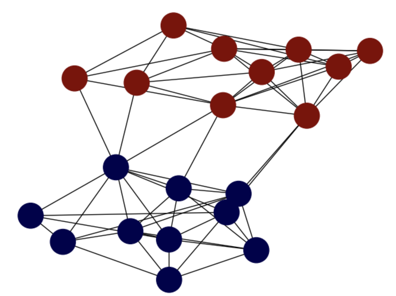
Fig. 6.8 SBM graph. Min-cut optimal partition .

A bit more formally, let us define the \(\text{cut}(A,B)\) between the two subsets, \(A\) and \(B\), of a partition as the number of edges with different colors at their nodes:

\[ \text{cut}(A,B) = \sum_{u\in A,v\in B}e(u,v)\;\;\text{with}\;\; e(u,v)\in E\;. \]

The idea of min-cut is to find the partition \((A,B)\) minimizing \(\text{cut}(A,B)\). However, doing so is not enough because if a given node \(u\) has \(d_u=1\), we may consider the following partition: \(A =\{u\}\) and \(B = V - \{u\} = V - A\), leading to \(\text{cut}(A,B)=1\) which is minimal but non-sense.

Then, it seems more reasonable to force the partition to be balanced. This can be done in a simple way by minimizing the so called average cut or ratio cut \(\text{Rcut}(A,B)\):

\[ \text{Rcut}(A,B) = \frac{\text{cut}(A,B)}{|A|} + \frac{\text{cut}(A,B)}{|B|}\;, \]

where \(|A|\) and \(|B|\) are the number of nodes of \(A\) and \(B\) respectively, which are maximized as \(\text{cut}(A,B)\) is minimized.

However, as there are \(2^{|V|}\) partitions or ways of coloring \(|V|\) nodes with \(2\) colors, the ratio cut problem is NP-Hard and we can only have approximations.

6.2.2. The Fiedler vector

Encoding partitions. Given a partition \((A,B)\), since \(|A| + |B| = |V|\) we can encode it with a vector \(\mathbf{f}\) of length \(|V|\) whose entries \(\mathbf{f}(u)\in \{-1,1\}\) for \(u\in V\). For instance, consider the graph in Fig. 6.9 and its partition: \(A = \{2,6\}, B=\{1,3,4,5\}\).

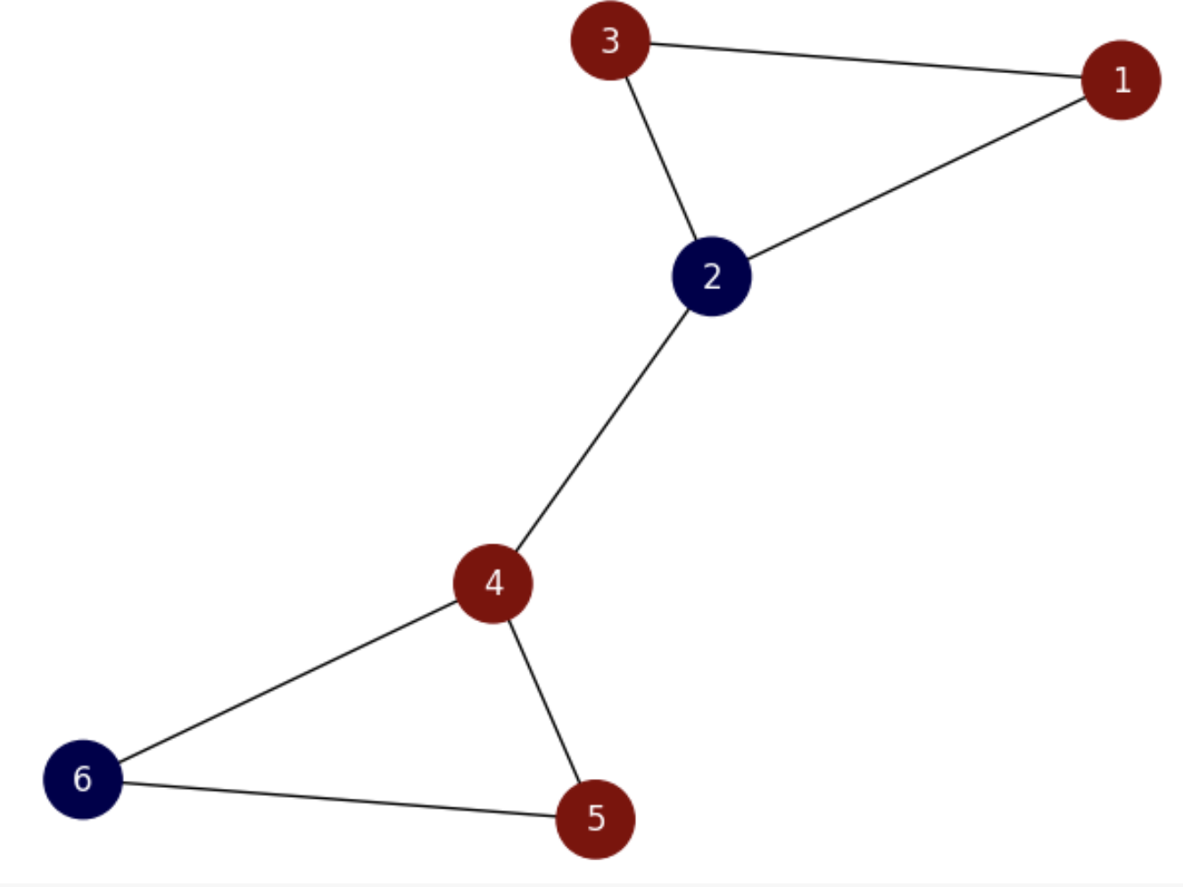
Fig. 6.9 Small graph with non-optimal partition.

The corresponding vector is

\[ \mathbf{f}=[+1\;-1\;+1\;+1\;+1\;-1]^T\;. \]

Then, for computing the ratio cut of the above partition we count the number of heterophilic edges (edges connecting nodes of different colors). They are \(E_{cut}=\{(1,2), (2,3), (2,4), (5,6)\}\). Then, \(\text{cut}(A,B)=|E_{cut}|=4\). Then, since \(|A|=2\) and \(|B|=4\) the ratio cut is

\[ \text{Rcut}(A,B) = \frac{|E_{cut}|}{|A|} + \frac{|E_{cut}|}{|B|} = \frac{4}{2} + \frac{4}{4} = 3\;. \]

Consider now the partition shown in Fig. 6.10.

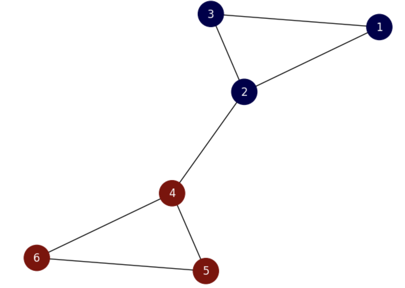
Fig. 6.10 Small graph with the optimal partition.

We have the vector

\[ \mathbf{f}=[-1\;-1\;-1\;+1\;+1\;+1]^T\; \]

and

\[ \text{Rcut}(A,B) = \frac{|E_{cut}|}{|A|} + \frac{|E_{cut}|}{|B|} = \frac{1}{3} + \frac{1}{3} = \frac{2}{3}\;, \]

which is clearly smaller than that of the previous partition: \(\frac{2}{3}<3\), showing that the ratio cut loss function measures the godness of a cut.

The ratio-cut loss function is, however, prone to degenerated solutions such as \(A=\{1,2,3,4,5,6\},\; B=\emptyset\) or vice versa:

\[ \text{Rcut}(A,B) = \frac{0}{|A|} + \frac{0}{|B|} = 0\;. \]

Consequently, any algorithm minimizing \(\text{Rcut}(A,B)\) must:

1. Find a vector \(\mathbf{f}\in\{-1,1\}^{|V|}\) encoding a partition \((A,B)\) such that minimizes \(\text{Rcut}(A,B)\).

2. The minimizing vector must be perpendicular/orthogonal to \(\mathbf{1}\) as well as different from \(\mathbf{0}\).

The last condition (orthogonality) ensures that the solution is quite different from the degenerated solution.

For instance,

\[ \mathbf{f}=[-1\;-1\;-1\;+1\;+1\;+1]^T\; \]

is orthogonal to \(\mathbf{1}\) since the dot product \(\mathbf{f}\cdot\mathbf{1}=0\). However,

\[ \mathbf{f}=[+1\;-1\;+1\;+1\;+1\;-1]^T\;. \]

is not orthogonal to \(\mathbf{1}\) since \(\mathbf{f}\cdot\mathbf{1}=4-2=2\neq 0\).

Continuous relaxation. Due to the NP hardness of the ratio-cut problem, instead of looking for discrete solutions, \(\mathbf{f}\in\{-1,1\}^{|V|}\) we must relax the vector space to allow \(\mathbf{f}\in [-1,1]^{|V|}\). This strategy is quite common in AI and it is called continuous relaxation. The main idea is that vectors with continuous entries are easier to be manipulated by algebraic techqiques so that they become an approximation of their discrete counterparts (relaxation really means “approximation”).

Miroslav Fiedler, while reasoning on how to use linear algebra to characterize the connectivity of graphs proposed the following loss equivalent to the ratio-cut:

\[ \lambda = |V|\cdot \left\{\frac{\sum_{u\sim v}(\mathbf{f}(u)-\mathbf{f}(v))^2}{\sum_{u,v}(\mathbf{f}(u)-\mathbf{f}(v))^2}\;: \mathbf{f}\neq\mathbf{0},\mathbf{f}\neq c\cdot\mathbf{1},c\in\mathbb{R}\right\}\;, \]

where the notation \(u\sim v\) means that “\(u\) and \(v\) are neighbors”. As a result, if \(\mathbf{f}\in\{-1,1\}^{|V|}\), the numerator of the above loss simply counts how many heterophilic edges do we have. The denominator counts how many heterophilic edges we would have if the graph were complete.

The correspondence of \(\lambda\) with the ratio cut loss is very interesting. Actually, all we have to do is to operate on the denominator as follows:

1. Use the Lagrange identity, which is valid for any vector \(\mathbf{f}\), to expand the denominator

\[ \frac{1}{2}\sum_{u,v}(\mathbf{f}(u)-\mathbf{f}(v))^2 = |V|\sum_{u}\mathbf{f}(u)^2 - \left(\sum_{u}\mathbf{f}(u)\right)^2\;. \]

2. Since the orthogonality of \(\mathbf{f}\) to \(\mathbf{1}\) means that \(\sum_{u}\mathbf{f}(u)=0\), the Lagrange identity becomes:

\[ \sum_{u,v}(\mathbf{f}(u)-\mathbf{f}(v))^2 = 2|V|\sum_{u}\mathbf{f}(u)^2. \]

3. Look now at the ratio cut and group the two fractions into a single one:

\[\begin{split} \begin{align} \text{Rcut}(A,B) &= \frac{|E_{cut}|}{|A|} + \frac{|E_{cut}|}{|B|}\\ &= \frac{|B|\cdot |E_{cut}| + |A|\cdot |E_{cut}|}{|A|\cdot|B|}\\ &= \frac{(|A|+|B|)\cdot |E_{cut}|}{|A|\cdot|B|}\\ &= \frac{|V|\cdot |E_{cut}|}{|A|\cdot|B|}\\ \end{align}\;. \end{split}\]

Now, setting \(|E_{cut}|=\sum_{u\sim v}(\mathbf{f}(u)-\mathbf{f}(v))^2\) and considering that \(\sum_{u}\mathbf{f}(u)^2\le |V|\) for \(\mathbf{f}\in [-1,1]^{|V|}\), we have that

\[ \lambda\le\text{Rcut}(A,B) \]

that is the loss \(\lambda\) is even more restrictive than the ratio cut loss!

Exercise. In order to better understand the ratio-cut function, let us illustrate how it applies to partition a complete graph \(K_n\), with \(n=5\) (without self-loops).

See Fig. 6.11 where the red curves defines in each case, what nodes are included in the subset \(A\) and what belong to its complementary \(B=\bar{A}\). Although theoretically we have \(2^{5}-2\) partitions (discounting \(\emptyset\) and \(V\)) for this graph, we really have \(4\) different partitions: respectively with one, two, three and four elements. From left to rigth we have four partitions \(A_i\): \(A_1=\{3\}\), \(A_2=\{3,1\}\), \(A_3=\{3,1,0\}\), and \(A_4=\{3,1,0,2\}\).

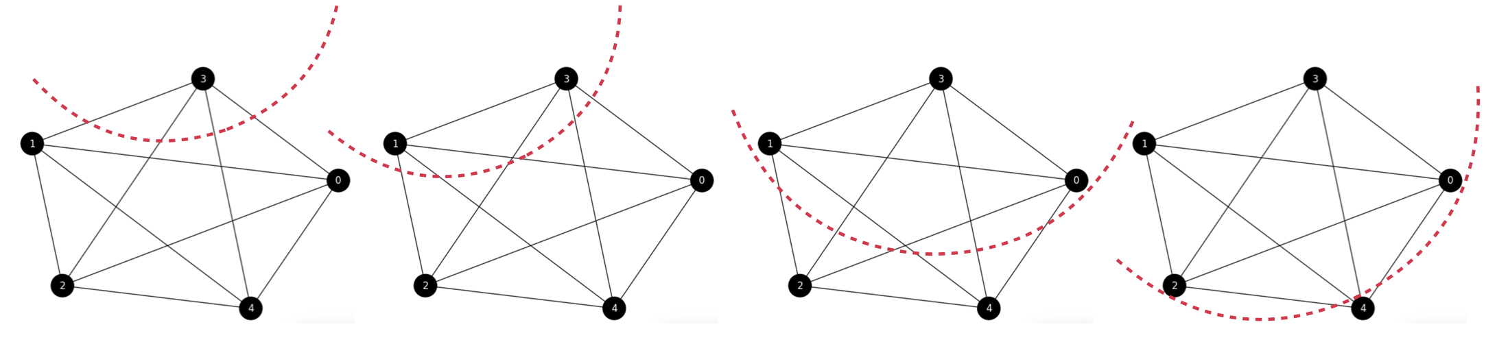
Fig. 6.11 From left to right: \((A_1,B_1)\), \((A_2,B_2)\), \((A_3,B_3)\) and \((A_4,B_4)\). All the cuts in \(K_n\) result from partitions which are equally optimal!

Let us compute the ratio-cut loss for each partition:

\( \begin{align} \text{cut}(A_1,B_1)=1\cdot 4\;\Rightarrow \text{Rcut}(A_1,B_1) = \frac{4}{|A_1|} + \frac{4}{|B_1|} = \frac{4}{1} + \frac{4}{4} = 5\\ \text{cut}(A_2,B_2)=2\cdot 3\;\Rightarrow \text{Rcut}(A_2,B_2) = \frac{6}{|A_2|} + \frac{6}{|B_2|} = \frac{6}{2} + \frac{6}{3} = 5\\ \text{cut}(A_3,B_3)=3\cdot 2\;\Rightarrow \text{Rcut}(A_3,B_3) = \frac{6}{|A_3|} + \frac{6}{|B_3|} = \frac{6}{3} + \frac{6}{2} = 5\\ \text{cut}(A_4,B_4)=4\cdot 1\;\Rightarrow \text{Rcut}(A_4,B_4) = \frac{4}{|A_4|} + \frac{4}{|B_4|} = \frac{4}{1} + \frac{4}{4} = 5\\ \end{align} \)

As a result, all the ratio cuts are equal! Why?

Consider the general case \(K_n=(V,E)\) with \(n\) nodes. Each node in \(K_n\) is connected to \(n-1\) nodes (remember that we have excluded self-loops).

Then if a subset \(A_k\subset V\) has \(k\) nodes, we have that \(B_k=V - A_k\) has \(n-k\) nodes. Since every node in \(A_k\) is linked (in this graph) with any node in \(B_k\) we have that

\( \text{cut}(A_k,B_k)=k\cdot(n-k)\;. \)

which results in

\( \text{Rcut}(A_k,B_k)=\frac{k\cdot(n-k)}{|A_k|} + \frac{k\cdot(n-k)}{|B_k|} = \frac{k\cdot(n-k)}{k} + \frac{k\cdot(n-k)}{(n-k)} = n - k + k = n\;. \)

Then, the ratio cut for all the cuts in \(K_n\) is always \(n\).

6.2.3. The Laplacian and Courant-Fischer

One of the most interestings discoveries of spectral theory is that for minimizing \(\lambda\) we only need to interpret it as the eigenvalue of \(\mathbf{f}\) which is an eigenvector of a symmetric matrix called the Laplacian.

The Laplacian of a graph \(G=(V,E)\), that we denote as \(\triangle\), is the matrix resulting for subtracting to the degree matrix the adjacency matrix of the graph:

\[ \triangle = \mathbf{D}-\mathbf{A}\;. \]

That is, in the diagonal of \(\triangle\) we have the degrees \(d_u\) of all the nodes \(u\in V\) and in the off-diagonal we have the negative of the adjacencies \(-a_{uv}\).

For our example graph, in Fig. 6.9 and Fig. 6.10, we have:

\[\begin{split} \triangle = \begin{bmatrix} \mathbf{d}_1 = 2 & -a_{12}=-1 & -a_{13}=-1 & -a_{14}=0 & -a_{15}=0 & -a_{16}=0\\ -a_{21}=-1 & \mathbf{d}_2 = 3 & -a_{23}=-1 & -a_{24}=-1 & -a_{25}=0 & -a_{26}=0\\ -a_{31}=-1 & -a_{32}=-1 & \mathbf{d}_3 = 2 & -a_{34}=0 & -a_{35}=0 & -a_{36}=0\\ -a_{41}=0 & -a_{42}=-1 & -a_{43}=0 & \mathbf{d}_4 = 3 & -a_{45}=-1 & -a_{46}=-1\\ -a_{51}=0 & -a_{52}=0 & -a_{53}=0 & -a_{54}=-1 & \mathbf{d}_5 = 2 & -a_{56}=-1\\ -a_{61}=0 & -a_{62}=0 & -a_{63}=0 & -a_{64}=-1 & -a_{65}=-1 & \mathbf{d}_6 = 2\\ \end{bmatrix} \end{split}\]

i.e.

\[\begin{split} \triangle = \begin{bmatrix} \mathbf{2} & -1 & -1 & 0 & 0 & 0\\ -1 & \mathbf{3} & -1 & -1 & 0 & 0\\ -1 & -1 & \mathbf{2} & 0 & 0 & 0\\ 0 & -1 & 0 & \mathbf{3} & -1 & -1\\ 0 & 0 & 0 & -1 & \mathbf{2} & -1\\ 0 & 0 & 0 & -1 & -1 & \mathbf{2}\\ \end{bmatrix} \end{split}\]

Some properties:

1. The Laplacian is usually considered the derivative operator in the graph domain (this is why we use the notation \(\triangle\)). Actually for any vector \(\mathbf{f}\in\mathbb{R}^{|V|}\) we have:

\[ \triangle\mathbf{f} = \sum_{u\sim v}\mathbf{f}(u)-\mathbf{f}(v)\;. \]

Actually, in the previous example we have:

\[\begin{split} \triangle\mathbf{f} = \begin{bmatrix} \mathbf{2} & -1 & -1 & 0 & 0 & 0\\ -1 & \mathbf{3} & -1 & -1 & 0 & 0\\ -1 & -1 & \mathbf{2} & 0 & 0 & 0\\ 0 & -1 & 0 & \mathbf{3} & -1 & -1\\ 0 & 0 & 0 & -1 & \mathbf{2} & -1\\ 0 & 0 & 0 & -1 & -1 & \mathbf{2}\\ \end{bmatrix} \begin{bmatrix} \mathbf{f}(1)\\ \mathbf{f}(2)\\ \mathbf{f}(3)\\ \mathbf{f}(4)\\ \mathbf{f}(5)\\ \mathbf{f}(6)\\ \end{bmatrix} = \begin{bmatrix} \mathbf{f}(1)-\mathbf{f}(2) + \mathbf{f}(1)-\mathbf{f}(3)\\ \mathbf{f}(2) - \mathbf{f}(1) + \mathbf{f}(2) - \mathbf{f}(3) + \mathbf{f}(2) - \mathbf{f}(4)\\ \mathbf{f}(3) - \mathbf{f}(1) + \mathbf{f}(3) - \mathbf{f}(2) \\ \mathbf{f}(4) - \mathbf{f}(2) + \mathbf{f}(4) - \mathbf{f}(5) + \mathbf{f}(4) - \mathbf{f}(6)\\ \mathbf{f}(5) - \mathbf{f}(4) + \mathbf{f}(5) - \mathbf{f}(6)\\ \mathbf{f}(6) - \mathbf{f}(4) + \mathbf{f}(6) - \mathbf{f}(5)\\ \end{bmatrix} \end{split}\]

2. The Laplacian is an harmonic operator, i.e. it satisfies that

\[ \mathbf{f}(u)=\frac{1}{d_u}\sum_{v\sim u}f(v)\;. \]

and you can check this at any row of \(\triangle\mathbf{f}\).

3. The Laplacian is linked with the \(\lambda\) loss as follows:

\[ \mathbf{f}^T\triangle\mathbf{f} = \frac{1}{2}\sum_{u\sim v}(\mathbf{f}(u)-\mathbf{f}(v))^2 \]

In order to visualize this, let us consider the product of \(\mathbf{f}^T\) and \(\triangle\mathbf{f}\) in the example:

\[\begin{split} \begin{bmatrix} \mathbf{f}(1) & \mathbf{f}(2) & \mathbf{f}(3) & \mathbf{f}(4) & \mathbf{f}(5) & \mathbf{f}(6) \end{bmatrix} \begin{bmatrix} \mathbf{f}(1)-\mathbf{f}(2) + \mathbf{f}(1)-\mathbf{f}(3)\\ \mathbf{f}(2) - \mathbf{f}(1) + \mathbf{f}(2) - \mathbf{f}(3) + \mathbf{f}(2) - \mathbf{f}(4)\\ \mathbf{f}(3) - \mathbf{f}(1) + \mathbf{f}(3) - \mathbf{f}(2) \\ \mathbf{f}(4) - \mathbf{f}(2) + \mathbf{f}(4) - \mathbf{f}(5) + \mathbf{f}(4) - \mathbf{f}(6)\\ \mathbf{f}(5) - \mathbf{f}(4) + \mathbf{f}(5) - \mathbf{f}(6)\\ \mathbf{f}(6) - \mathbf{f}(4) + \mathbf{f}(6) - \mathbf{f}(5)\\ \end{bmatrix} \end{split}\]

from this product of \((1\times |V|)(|V|\times 1)\) we get a scalar as follows:

\[ \mathbf{f}(1)\triangle\mathbf{f} + \mathbf{f}(2)\triangle\mathbf{f} + \ldots + \mathbf{f}(|V|)\triangle\mathbf{f}\;. \]

and plugging in \(\triangle\mathbf{f}=\sum_{u\sim v}\mathbf{f}(u)-\mathbf{f}(v)\) we have

\[ \mathbf{f}(1)\sum_{1\sim v}\mathbf{f}(1)-\mathbf{f}(v) + \mathbf{f}(2)\sum_{2\sim v}\mathbf{f}(2)-\mathbf{f}(v) + \ldots + \mathbf{f}(n)\sum_{n\sim v}\mathbf{f}(n)-\mathbf{f}(v)\;. \]

where \(n=|V|\). This leads to

\[ \mathbf{f}(1)\sum_{1\sim v}\mathbf{f}(1)^2-\mathbf{f}(1)\mathbf{f}(v) + \sum_{2\sim v}\mathbf{f}^2(2)-\mathbf{f}(2)\mathbf{f}(v) + \ldots + \sum_{n\sim v}\mathbf{f}(n)^2-\mathbf{f}(n)\mathbf{f}(v)\;. \]

For a any edge, say \(e=(u,v)\) the above sum contains \(f(u)^2 + f(v)^2 - 2f(u)f(v) = (f(u)-f(v))^2\).

See for instance, \(e=(1,2)\) which involves nodes \(1\) and \(2\). From the above sum (see also the two first elements of \(\triangle\mathbf{f}\)) we have:

\[ f(1)^2 - f(1)f(2) + f(1)^2 - f(1)f(3) \]

and

\[ f(2)^2 - f(2)f(1) + f(2)^2 - f(2)f(3) + f(2)^2 - f(2)f(4) \]

For \(e=(1,2)\) we take

\[ f(1)^2 - f(1)f(2)-f(2)f(1) + f(2)^2 = (f(1) - f(2))^2 \]

and there are more terms for \(e=(2,1)\) and similarly for the remaining edges thus leading to

\[ 2\sum_{u\sim v}(f(u)-f(v))^2\;. \]

By the Lagrange identity we know that

\[ \sum_{u,v}(\mathbf{f}(u)-\mathbf{f}(v))^2 = 2|V|\sum_{u}\mathbf{f}(u)^2. \]

As a result, we have that

\[ \lambda = \left\{\frac{\sum_{u\sim v}(\mathbf{f}(u)-\mathbf{f}(v))^2}{\sum_{u}\mathbf{f}(u)^2}\;: \mathbf{f}\neq\mathbf{0},\mathbf{f}\neq c\cdot\mathbf{1},c\in\mathbb{R}\right\}\;. \]

Since \(\sum_{u}\mathbf{f}(u)^2=\mathbf{f}^T\mathbf{f}=||\mathbf{f}||^2\) is the squared modulus of \(\mathbf{f}\), we have a more compact definition of \(\lambda\):

\[ \lambda = \left\{\frac{\mathbf{f}^T\triangle\mathbf{f}}{\mathbf{f}^T\mathbf{f}}\;: \mathbf{f}\neq\mathbf{0},\mathbf{f}\neq c\cdot\mathbf{1},c\in\mathbb{R}\right\}\;. \]

Courant-Fischer Theorem. Given an \(n\times n\) symmetric matrix \(\triangle\), it has \(n\) real eigenvalues \(\lambda_1\le\lambda_2\le\ldots\le\lambda_n\) with their associated real-valued eigenvectors \(\phi_1,\phi_2,\ldots,\phi_n\) satisfying \(\triangle\phi_i = \lambda_i\phi_i\) also satisfies:

\[\begin{split} \begin{align} \lambda_1 &= \min_{\mathbf{f}\neq 0}\frac{\mathbf{f}^T\triangle\mathbf{f}}{\mathbf{f}^T\mathbf{f}}\Rightarrow \mathbf{f}=\phi_1\\ \lambda_2 &= \min_{\mathbf{f}\neq 0, \mathbf{f}\perp \phi_1}\frac{\mathbf{f}^T\triangle\mathbf{f}}{\mathbf{f}^T\mathbf{f}}\Rightarrow \mathbf{f}=\phi_2\\ \lambda_3 &= \min_{\mathbf{f}\neq 0, \mathbf{f}\perp \{\phi_1,\phi_2\}}\frac{\mathbf{f}^T\triangle\mathbf{f}}{\mathbf{f}^T\mathbf{f}}\Rightarrow \mathbf{f}=\phi_3\\ & \ldots\\ \lambda_n &= \min_{\mathbf{f}\neq 0, \mathbf{f}\perp \{\phi_1,\phi_2,\ldots,\phi_{n-1}\}}\frac{\mathbf{f}^T\triangle\mathbf{f}}{\mathbf{f}^T\mathbf{f}}\Rightarrow \mathbf{f}=\phi_n\\ \end{align} \end{split}\]

Looking at the eigenvectors, they are interpreted as real-valued functions \(\phi:V\rightarrow\mathbb{R}\) and eigenvalues are the variations of these functions over the graph \(G=(V,E)\).

Laplacian spectrum and eigenvectors. From the above theorem we have that for the Laplacian \(\triangle\):

1. \(\lambda_1=0\). Since the rows of the Laplacian add \(0\), the smallest eigenvalue of the Laplacian is \(\lambda_1=0\) with eigenvector \(\phi=\mathbf{1}\).

\[ \triangle\phi_1 = \lambda_1\phi_1\Rightarrow \triangle\mathbf{1} = 0\cdot \mathbf{1}\;. \]

2. If the graph is connected, \(\lambda_2 = \min \lambda\) (minimum of the Fiedler loss). As a result, \(\lambda_2\), the Fiedler value can be interpreted as the minimal non-zero variance achievable for functions which are perpendicular to \(\mathbf{1}\), and the Fiedler vector is that function..

For instance, the Fiedler vector for the small example is mapped on the graph in Fig. 6.12.

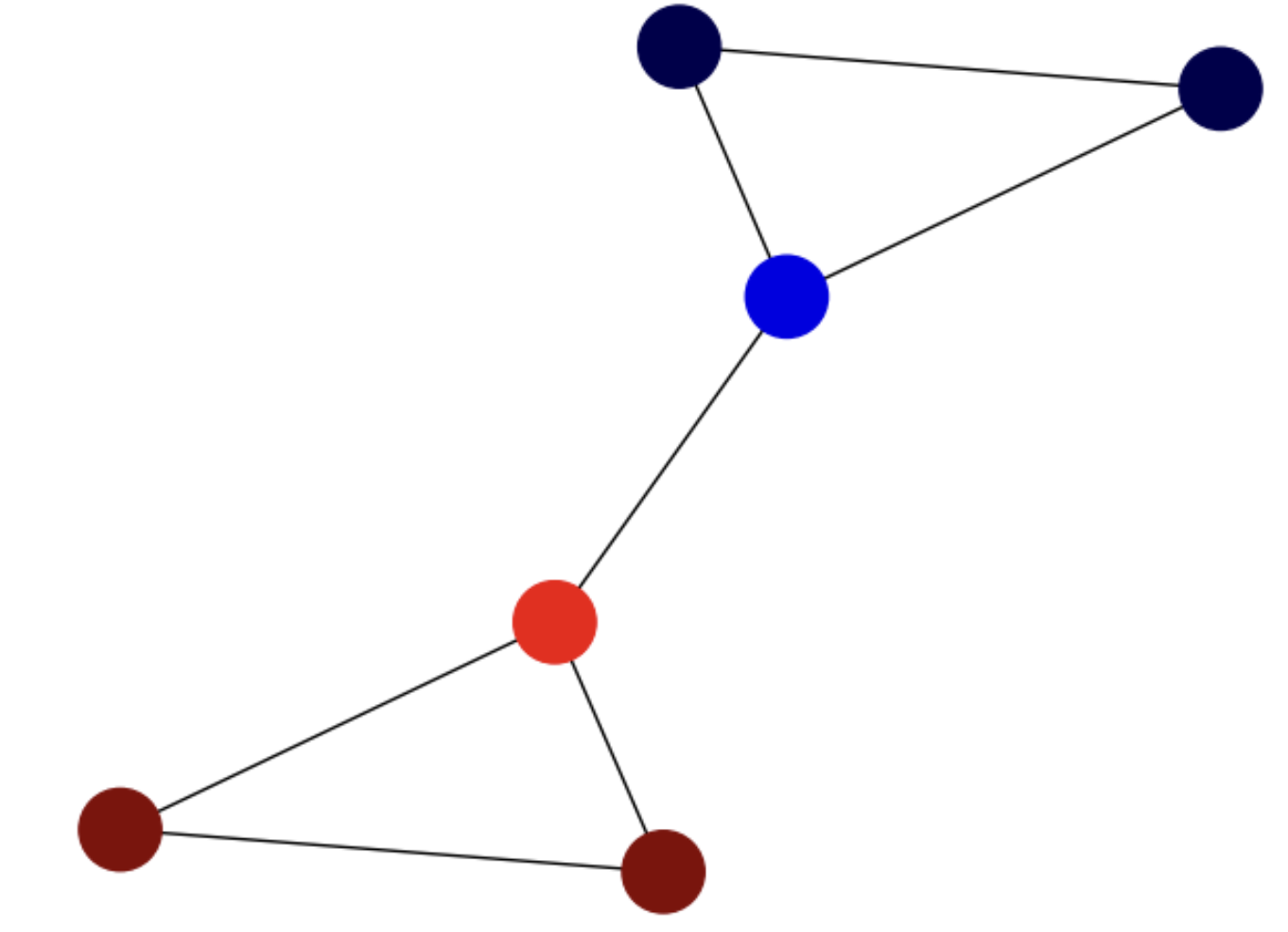
Fig. 6.12 Small graph and its Fiedler vector mapped on the nodes.

In the above graph, we have:

\[ \lambda_2=0.438,\;\; \phi_2^T=[-0.464\; -0.260\; -0.464\; +0.260\; +0.464\;+0.464]\;, \]

where we have part of the components negative (corresponding to \(-1\)) and part of them positive (corresponding to \(+1\)), thus approximating a partition in time \(O(n^3)\), the one needed to solve a system.

Interestingly the components \(\phi_2(2)\) and \(\phi_2(4)\) have the smaller absolute value although they are defining an heterophilic edge. This is a limitation of the continuous relaxation.

The Fiedler vector for the SBM example is mapped on the graph in Fig. 6.13.

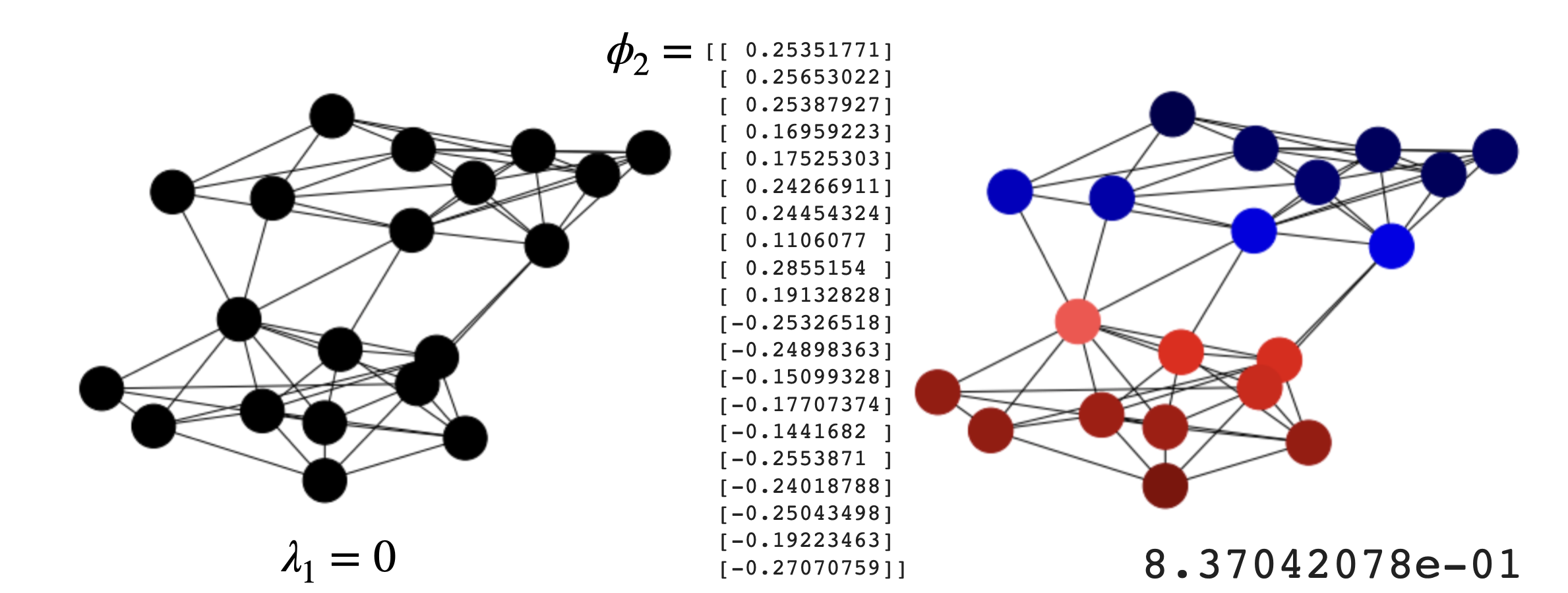
Fig. 6.13 SBM and its Fiedler vector mapped on the nodes.

The Spectrum. The spectrum of \(\triangle\) is the collection of \(n\) eigenvalues \(\lambda_1\le\lambda_2\le\ldots\le\lambda_n\). They are not-decreasing because they summarize the increasing variability of their respective eigenvectors mapped on the nodes of the graph (see Fig. 6.14).

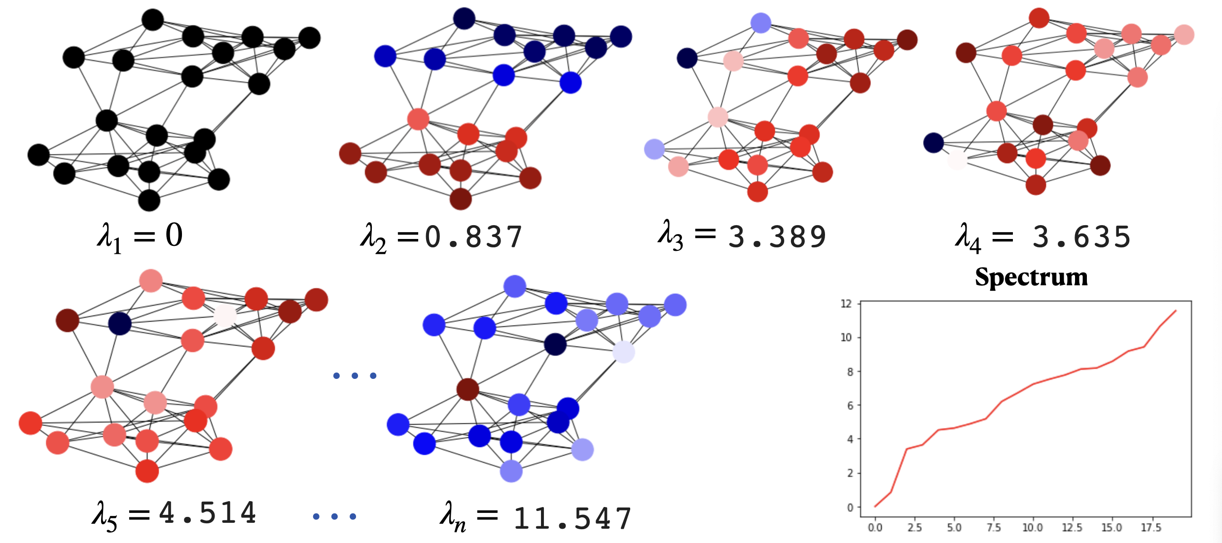
Fig. 6.14 SBM spectrum and its associated eigenvectors.

6.2.4. The Spectral Theorem

The Spectral Theorem. One of the most interesting facts of spectral theory in general is that, despite not the full spectrum and eigenvectors are necessary in AI, any symmetric and square matrix can be decomposed as follows:

\[ \triangle = \lambda_1\phi_1\phi_1^T + \lambda_2\phi_2\phi_2^T + \ldots + \lambda_n\phi_n\phi_n^T\;. \]

More compactly,

\[ \triangle = \Phi\Phi^T = \sum_{i=1}^n\lambda_i\phi_i\phi_i^T\;, \]

where the columns of \(\Phi\) are \(\phi_1,\phi_2,\ldots,\phi_n\).

The meaning of this theorem is that the matrix (\(\triangle\) for instance) can be perfectly decomposed (without loss of information) as a linear combination of \(n\) matrices \(\phi_i^T\phi_i\), each one defined by an eigenctor, and the coefficients of this linear combination are the coefficients of the eigenvalues.

However, if we do not have the full set of eigenvectors but a small number \(k<n\) of them, all we do is to approximate the matrix (the Laplacian of the graph in the case of \(\triangle\)). The error of the approximation is given by the sum of the absolute values of the discarded eigenvalues or modes.

In graph spectral theory, it is quite common to retain (or compute) only the smallest \(k\) eigenvectors of the Laplacian \(\triangle\):

\[ \triangle = \sum_{i=1}^k\lambda_i\phi_i\phi_i^T\;. \]

Consider, for instance the SBM example developed in this topic. In Fig. 6.15 we show the Lapacian matrix \(\triangle\) (top-left) and its eigenvectors \(\phi_1,\phi_2,\ldots,\phi_n\) (columns from left to right). The mapping of each eigenvector on the graph and the Laplacian spectrum are shown in Fig. 6.14.

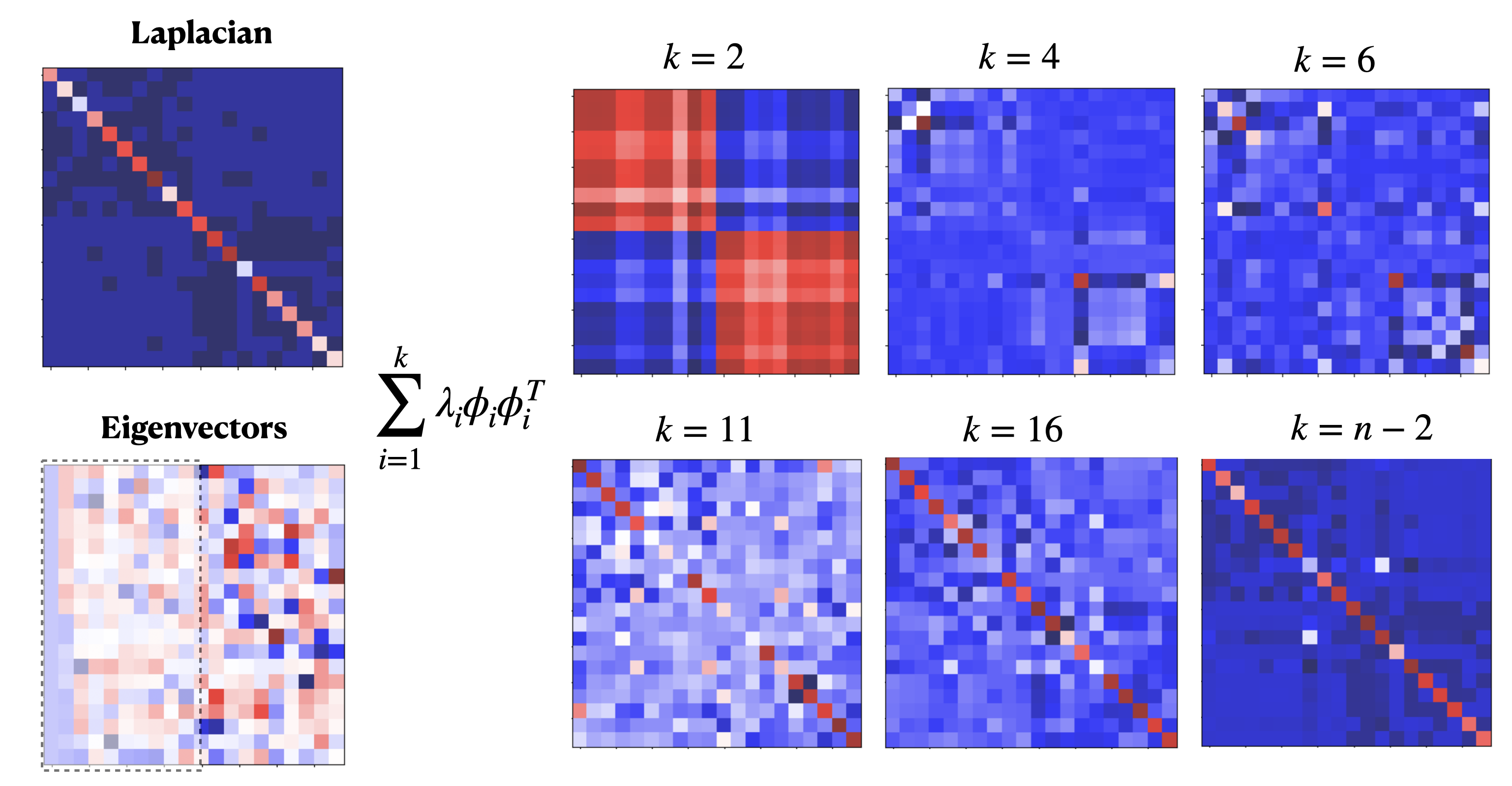
Fig. 6.15 SBM eigenvectors and reconstruction.

Then, looking at the matrix of eigenvectors \(\Phi\) (bottom-left), the first one \(\phi_1\) is constant \(\mathbf{1}\).

First-order approximation. For \(k=1\) we have the appoximation:

\[ \triangle = \lambda_1\phi_1\phi_1^T = 0\cdot \mathbf{1}\mathbf{1}^T = \mathbf{0}\;, \]

i.e. the first-order approximation of the Laplacian is a matrix of ones (all the elements in the matrix are equally important) weighted by zero. We know that this is highly incorrect since the diagonal must allocate the node degrees. This is exactly what the product by \(\lambda_1=0\) means!

Second-order approximation. The second eigenvector, the approximation of the Fiedler vector, partitions the graph into two communities and this is why the second-order approximation \(k=2\):

\[ \triangle = \lambda_1\phi_1\phi_1^T + \lambda_2\phi_2\phi_2^T \]

captures the dominant information in the graph: the two communities in the SBM. Remember that red means high positive value and blue high negative. Then for \(k=2\) we only know that there is a high probability that half of the nodes belong to a community and the other half to another one.

Mid-order approximation. For \(k>2\) we observe that few elements in the diagonal are captured. See for instance the red corners in \(k=4\) and \(k=6\). These two nodes belong to inter-class edges. They are also linked with nodes of same community: remember that adjacency in the Laplacian is \(-1\) (encoded by dark blue).

High-order approximation. See that for \(k\ge 11\) degree information is recovered before the full (negative) adjacency emerges!

Therefore, the logical order of emerging info during the approximation is:

1. Cluster structure of the graph.

2. Important nodes (intrer-class).

3. Degree info.

4. Negative adjacency.

For a better understanding of these steps we propose a small exercise.

Exercise. Let us consider the small SBM whose Fiedler vector is shown in Fig. 6.12. We only have \(\lambda_1,\phi_1\) and \(\lambda_2,\phi_2\). Then, from:

\( \begin{align} &\lambda_1 = 0.0\;\;\phi_1 = [+1.0\; +1.0\; +1.0\; +1.0\; +1.0\; +1.0]^T\\ &\lambda_2=0.4\;\;\phi_2 =[-0.4\; -0.3\; -0.4\; +0.3\; +0.4\;+0.4]\; \end{align} \)

apply the spectral theorem to approximate the Laplacian matrix using the information given. We have:

\( \triangle \approx \lambda_1\phi_1\phi_1^T + \lambda_2\phi_2\phi_2^T \)

Since \(\lambda_1=0\), we have:

\( \triangle \approx \lambda_2\phi_2\phi_2^T\;. \)

\( \phi_2\phi_2^T = \begin{bmatrix} -0.4\\ -0.3\\ -0.4\\ +0.3\\ +0.4\\ +0.4 \end{bmatrix} \begin{bmatrix} -0.4 & -0.3 & -0.4 & +0.3 & +0.4 & +0.4 \end{bmatrix} \)

\( \phi_2\phi_2^T = \begin{bmatrix} 0.16 & 0.12 & 0.16 & -0.12 & -0.16 & -0.16\\ 0.12 & 0.09 & 0.12 & -0.09 & -0.12 & -0.12\\ 0.16 & 0.12 & 0.16 & -0.12 & -0.16 & -0.16\\ -0.12 & -0.09 & -0.12 & 0.09 & 0.12 & 0.12\\ -0.16 & -0.12 & -0.16 & 0.12 & 0.16 & 0.16\\ -0.16 & -0.12 & -0.16 & 0.12 & 0.16 & 0.16\\ \end{bmatrix} \)

\( \lambda_2\phi_2\phi_2^T = \begin{bmatrix} 0.064 & 0.048 & 0.064 & -0.048 & -0.064 & -0.064\\ 0.048 & 0.036 & 0.048 & -0.036 & -0.048 & -0.048\\ 0.064 & 0.048 & 0.064 & -0.048 & -0.064 & -0.064\\ -0.048 & -0.036 & -0.048 & 0.036 & 0.048 & 0.048\\ -0.064 & -0.048 & -0.064 & 0.048 & 0.064 & 0.064\\ -0.064 & -0.048 & -0.064 & 0.048 & 0.064 & 0.064\\ \end{bmatrix} \)

Then, with the first two eigenvalues and eigevectors all we can do is to capture the block structure (communities) in the SBM, as shown in Fig. 6.15. Look that the positive blocks (red in Fig. 6.15) correspond to the intra-class links inside the two communities, where the negative blocks correspond to inter-class edges!