7. Distances and Latent Spaces

7.1. Normalized Laplacian

7.1.1. Derivation

The normalized Laplacian \(\tilde{\triangle}\) is a slight modification of the Laplacian which was initially designed for relating the spectra of transition matrices and Laplacian matrices. Actually, the first chapters of the book of Fan Chung-Graham are a must for students interested in spectral graph theory, though the level is very top in mathematical terms. Herein we will refer to basic concepts for the perusal of AIers.

Derivation from the Transition. Remember the transition matrix of \(G=(V,E)\):

\[ \mathbf{P} = \mathbf{D}^{-1}\mathbf{A}\;\;\text{i.e.}\;\; p_{ij} = \frac{a_{ij}}{d_i}\;. \]

If \(\mathbf{P}\) is irreducible and aperiodic (for instance the one given by the Google matrix), we have that the spectrum (eigenvalues) of \(\mathbf{P}\) satisfy:

\[ 1=\lambda_1\ge\lambda_2\ge \ldots \ge \lambda_n>-1\;. \]

Let us now define the following matrix \(\tilde{\mathbf{P}}\) (which is different from \(\mathbf{P}\)):

\[ \tilde{\mathbf{P}} = \mathbf{D}^{-1/2}\mathbf{A}\mathbf{D}^{-1/2}\;, \]

where \(\mathbf{D}^{-1/2}\) is the diagonal matrix with elements \(1/\sqrt{d_i}\).

Then, the normalized Laplacian is given by

\[ \tilde{\triangle} = \mathbf{I} - \tilde{\mathbf{P}} = \mathbf{I} - \mathbf{D}^{-1/2}\mathbf{A}\mathbf{D}^{-1/2}\;, \]

where \(\mathbf{I}\) is the identity matrix of size \(|V|\). It turns out that if \(\lambda_k\) is an eigenvalue of \(\mathbf{P}\), then \(1 - \lambda_k\) is an eigenvalue of \(\tilde{\triangle}\) and vice versa.

Derivation from the Laplacian. In her book, Fan Chun approaches the normalized Laplacian in a different way. Consider now the (unnormalized) Laplacian

\[ \triangle = \mathbf{D} - \mathbf{A}\;. \]

Let us define \(\tilde{\triangle}\) as the pre-multiplication and post-multipliplication of \(\triangle\) by \(\mathbf{D}^{-1/2}\) (degree normalization):

\[\begin{split} \begin{align} \tilde{\triangle}=\mathbf{D}^{-1/2}\triangle \mathbf{D}^{-1/2} &= \mathbf{D}^{-1/2}(\mathbf{D} - \mathbf{A})\mathbf{D}^{-1/2}\\ &= \mathbf{D}^{-1/2}\mathbf{D}\mathbf{D}^{-1/2} - \mathbf{D}^{-1/2}\mathbf{A}\mathbf{D}^{-1/2}\\ &= \mathbf{I} - {D}^{-1/2}\mathbf{A}\mathbf{D}^{-1/2}\\ &= \mathbf{I} - \tilde{\mathbf{P}}\;. \end{align} \end{split}\]

Then, the component-wise structure of \(\tilde{\triangle}\) is

\[\begin{split} \tilde{\triangle}_{ij}= \begin{cases} -\frac{1}{\sqrt{d_i}\sqrt{d_j}}\;\text{if}\; (i,j)\in E \\[2ex] 1\;\text{if}\; i=j \;\text{and}\; d_i\neq 0\\[2ex] 0\; \text{otherwise}\;, \end{cases} \end{split}\]

i.e. in the diagonal we have \(\tilde{\triangle}_{ii}=1\) (normalized) and in the off-diagonal we will have \(-\frac{1}{\sqrt{d_id_j}}\).

Link between the eigenvectors. If \(\phi\) and \(\tilde{\phi}\) are respectively eigenvectors of \(\triangle\) and \(\tilde{\triangle}\), they are related by the equations: \(\tilde{\phi}=\mathbf{D}^{1/2}\phi\) and \(\phi=\mathbf{D}^{-1/2}\tilde{\phi}\):

\[\begin{split} \begin{align} \tilde{\triangle}\tilde{\phi} = \lambda\tilde{\phi}\; &\Rightarrow \mathbf{D}^{-1/2}\triangle\mathbf{D}^{-1/2}\tilde{\phi} = \lambda\tilde{\phi}\\ &\Rightarrow \mathbf{D}^{-1/2}\triangle\mathbf{D}^{-1/2}(\mathbf{D}^{1/2}\phi) = \lambda(\mathbf{D}^{1/2}\phi)\\ &\Rightarrow \mathbf{D}^{-1/2}\triangle\phi = \lambda\mathbf{D}^{1/2}\phi\\ &\Rightarrow \mathbf{D}^{1/2}\mathbf{D}^{-1/2}\triangle\phi = \mathbf{D}^{-1/2}\lambda\mathbf{D}^{1/2}\phi\\ &\Rightarrow \triangle\phi = \mathbf{D}^{1/2}\lambda\mathbf{D}^{1/2}\phi\\ &\Rightarrow \triangle\phi = \lambda\mathbf{D}\phi\;.\\ \end{align} \end{split}\]

In other words, the eigenvectors of \(\tilde{\triangle}\) are the generalized eigenvectors of \(\triangle\).

For instance, as \(\mathbf{1}\) is the eigenvector of \(\triangle\) with eigenvalue \(\lambda_1=0\), then \(\mathbf{D}^{1/2}\mathbf{1}\) is the corresponding eigenvector for \(\tilde{\triangle}\). This means that the Fiedler vector associated with the normalized Laplacian must be perpendicular to \(\mathbf{D}\mathbf{1}\).

7.1.2. Spectral properties of graphs

In general, using the normalized Laplacian we obtain more robust estimators and this is why some properties of the graph that can be identified simply by looking at the spectrum of \(\tilde{\triangle}\) are enunciated.

Let \(n=|V|\) in \(G=(V,E)\). Then:

1. Sum of spectra. The sum of all eigenvalues is \(\sum_i\lambda_i\le n\), with equality only if the graph is connected. The proof is trivial since the trace of the matrix (sum of the diagonal) satisfies \(\text{Tr}[\tilde{\triangle}]=\sum_{i}\lambda_i\).

2. Bound of the spectra. For all \(i\le n\) we have \(\lambda_i\le 2\), with \(\lambda_n=2\) only if a connected component of the graph is bipartite.

3. Extent of the spectra. A graph without isolated nodes satisfies \(\lambda_n\ge \frac{n}{n-1}\) with equality if the graph is complete (without self-loops).

4. Number of connected components. There are \(k\) connected components if \(\lambda_1=\lambda_2=\ldots=\lambda_k = 0\).

Algebraic connectivity \(\lambda_2\). The second smallest eigenvalue of \(\tilde{\triangle}\) (the Fiedler value) is one of the most informative since:

5. \(\lambda_2\le \frac{n}{n-1}\) with equality only if \(G\) is the complete graph (without self-loops)

6. \(\lambda_2<1\) if the \(G\) is not complete.

7. The diameter \(D\) of \(G\) (length of the shortest path between any pair of nodes) satisfies: \(\frac{1}{D\text{vol}G}<\lambda_2\).

Some examples of graph spectra (from Chung’s book):

• Complete graph \(K_n\)(without self-loops): is \(0\) and \(\frac{n}{n-1}\) (with multiplicity \(n-1\)).

• Star graph (hub) \(S_n\): is \(0\), \(1\) (with multiplicity \(n-2\)) and \(2\).

• Path graph \(P_n\): is \(1-\cos\frac{\pi k}{n-1}\) for \(k=0,1,\ldots,n-1\).

• Cycle graph \(C_n\): is \(1-\cos\frac{2\pi k}{n}\) for \(k=0,1,\ldots,n-1\).

The Complete Graph’s Spectrum. Fig. 7.1. We have analized the optimal ratio-cut solution for this graph in the previous topic and we realized that all the cuts have the same cost. This is why the non-trivial spectrum is \(\lambda_i=\frac{n}{n-1},\;i\ge 1\) which for \(n=5\) is \(\lambda_i=1.25,\;i\ge 1\). The non-trivial eigenvectors correspond to different solutions equally optimal.

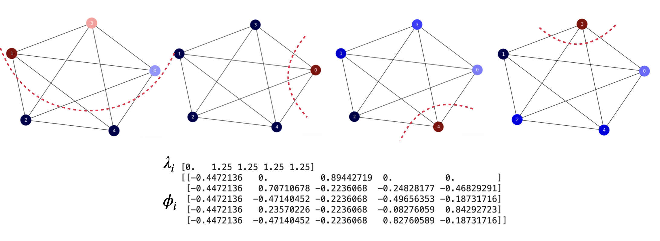
Fig. 7.1 \(K_5\). Normalized Laplacian’s spectrum and non-trivial eigenvectors.

The Star Graph’s Spectrum. Fig. 7.2. For the star graph, we can analyze a bit the optimal solution in terms of the ratio cut loss. To do that, for \(S_5\) (which has \(n=5\) nodes) let us generate partitions with \(0\), \(1\), \(2\), \(3\) nodes the same color as the central one.

• When only the central node has a different color than the remaining ones we have \(A_1=\{0\}\), \(B_1=\{1,2,3,4\}\) and

\[ \text{Rcut}(A_1,B_1) = \frac{\text{cut}(A_1,B_1)}{|A_1|} + \frac{\text{cut}(A_1,B_1)}{|B_1|} = \frac{4}{1} + \frac{4}{4} = 4 + \frac{4}{4} = 5\;. \]

• When the central node and 1 other one have the same color than the remaining ones we have, for instance, \(A_2=\{0,1\}\), \(B_2=\{2,3,4\}\). Then, \(\text{cut}(A_2,B_2)=|B_2|=3\). Then

\[ \text{Rcut}(A_2,B_2) = \frac{|B_2|}{|A_1|} + \frac{|B_2|}{|B_1|} = \frac{3}{2} + \frac{3}{3} = 1 + \frac{3}{2} = \frac{5}{2}=2.5\;. \]

• When the central node and 2 other nodes have the same color than the remaining ones we have, for instance, \(A_3=\{0,1,2\}\), \(B_3=\{3,4\}\). Then, \(\text{cut}(A_3,B_3)=|B_3|=2\). Then

\[ \text{Rcut}(A_3,B_3) = \frac{|B_3|}{|A_3|} + \frac{|B_3|}{|B_3|} = \frac{2}{3} + \frac{2}{2} = 1 + \frac{2}{3} = \frac{5}{2}=2.5\;. \]

• When the central node and 3 other nodes have the same color than the remaining ones we have, for instance, \(A_4=\{0,1,2,3\}\), \(B_4=\{4\}\). Then, \(\text{cut}(A_4,B_4)=|B_4|=1\). Then

\[ \text{Rcut}(A_4,B_4) = \frac{|B_4|}{|A_4|} + \frac{|B_4|}{|B_4|} = \frac{1}{4} + \frac{1}{1} = 1 + \frac{1}{4} = \frac{5}{4}=1.25\;. \]

Therefore, the best ratio-cut partition is \((A_4,B_4)\) (4 nodes with the same color and \(1\) different). Herein it is critical than one of the nodes with the same color is the central one. Otherwise we have the worse partition \((A_1,B_1)\). The other two partitions have the same cost and are intermediate solutions between the best and the worse partitions.

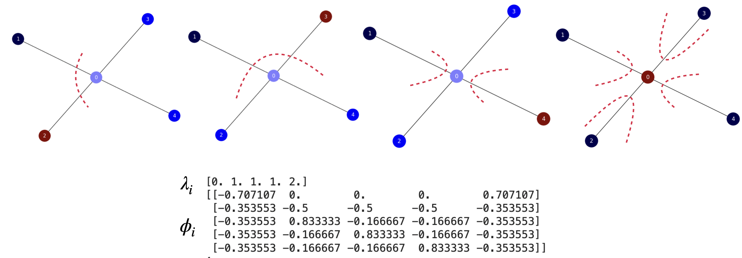
Fig. 7.2 \(S_5\). Normalized Laplacian’s spectrum and non-trivial eigenvectors.

However, the spectral approach misses the optimal solution \((A_4,B_4)\). The Fiedler vector (left-first in Fig. 7.2) is basically a permutation of the second and the third eigenvectors. All these eigenvectors have the same eigenvalue: \(1\); they encode the same solution: the one equalent to \((A_2,B_2)\) which is sub-optimal since its cost is \(2.5\).

Finally, the last eigenvector, which eigenvalue \(2\) encodes the worst solution \((A_1,B_1)\)

Despite not finding the optimal solution, given that spectral theory provides approximations, this is a good example of how spectral theory (which is a continuous maths tool) captures the combitorial nature of graph coloring (which is a discrete problem).

The Path Graph’s Spectrum. This graph also illustrated the combinatorial nature of spectral theory. In Fig. 7.3, we show the spectrum and non-trivial eigenvectors of \(P_5\).

In combinatorial terms, see that in a Path graph of \(n\) nodes we have \(n-1\) edges. As usual, we have \(2^n-2\) ways (removing \(\emptyset\) and \(V\)) of bi-partitioning this graph.

Since the ratio-cut prefers balanced cuts, the optimal solutions (there may be more than one due to the symmetry of the graphs) correspond to having \(\text{cut}(A_i,B_i)=1\) and \(|A_i|=\lceil n/2\rceil\) (ceil of the integer division). As a result

\[ \text{Rcut}(A_i,B_i) = \frac{1}{\lceil n/2\rceil} + \frac{1}{n - \lceil n/2\rceil}\;. \]

For \(P_5\), since \(n=5\) is odd then \(\lceil n/2\rceil=\lceil 5/2\rceil=3\) and the optimal ratio-cut loss is:

\[ \text{Rcut}(A_1,B_1) = \frac{1}{3} + \frac{1}{5 - 3} = \frac{1}{3} + \frac{1}{2} = \frac{5}{6}=0.83\;. \]

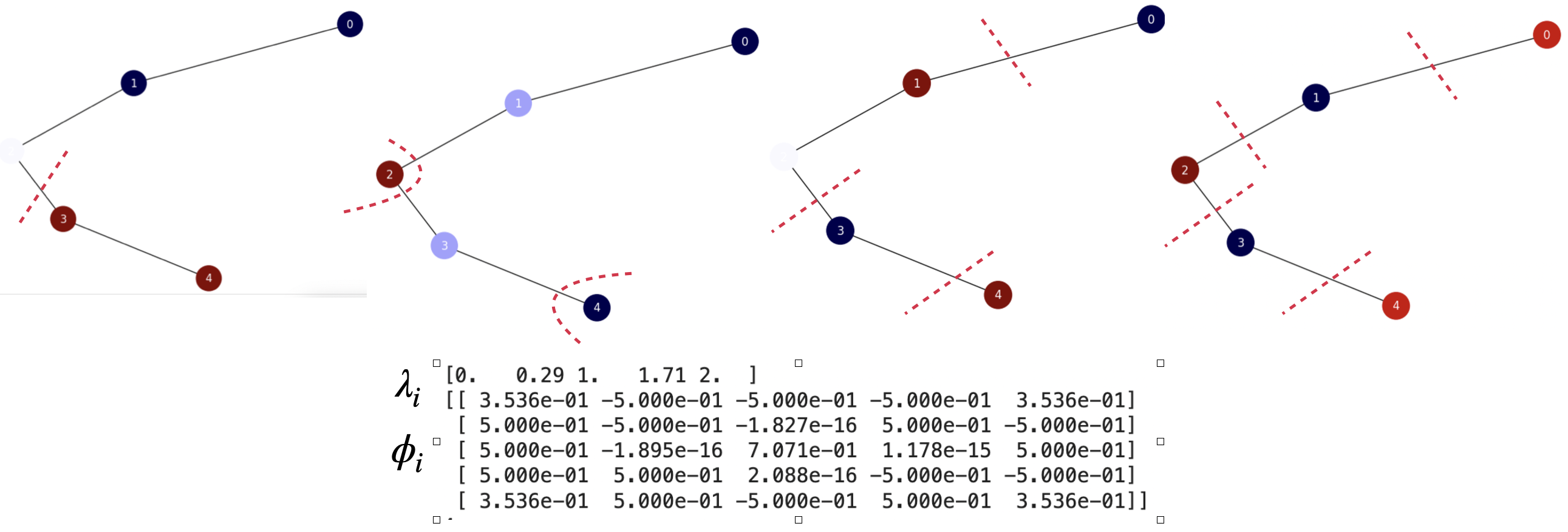
Fig. 7.3 \(P_5\). Normalized Laplacian’s spectrum and non-trivial eigenvectors.

In this case, the spectral approximation return the optimal solution \((A_1,B_1)\) (see the Fiedler vector in the figure, with eigenvalue \(0.29\)). The remaning eigenvalues are greater or equal than \(1\) and encode increasingly non-optimal solutions.

For instance, the solution encodes by the third smallest eigenvector of the normalized Laplacian is \(A_2=\{0,1,3\}\) and \(B_2=\{2,4\}\) and it has \(\text{cut}(A_2,B_2)=3\). Then:

\[ \text{Rcut}(A_2,B_2) = \frac{3}{3} + \frac{3}{2} = 1 + \frac{3}{2} = \frac{5}{2}=2.5\;. \]

The one corresponding to the fourth smalles eigenvector is \(A_3=\{0,3\}\), \(B_3=\{1,2,4\}\) with \(\text{cut}(A_3,B_3)=3\) and

\[ \text{Rcut}(A_3,B_3) = \frac{3}{2} + \frac{3}{3} = 1 + \frac{3}{2} = \frac{5}{2}=2.5\;. \]

Finally, the eigenector with the largest eigenvalue corresponds to \(A_4=\{0,2,4\}\) and \(B_4=\{1,3\}\) with the largest cut: \(\text{cut}(A_3,B_3)=4\) and

\[ \text{Rcut}(A_4,B_4) = \frac{4}{3} + \frac{4}{2} = \frac{4}{3} + \frac{4}{2} = \frac{8+12}{6}=\frac{20}{6}=3.3\;. \]

Therefore, in this case spectral theory grades the discrete solutions exactly!

The Cycle Graph’s Spectrum. Finally, the Cycle graph is a variant of the Path graph where the end node and the start one are linked. This simplifies the analysis a lot. As we can see in Fig. 7.4 the Fiedler vector encodes the optimal solution \(A_1=\{0,1,4\}\), \(B_1=\{2,3\}\), with \(\text{cut}(A_1,B_1)=2\). Then

\[ \text{Rcut}(A_1,B_1) = \frac{2}{3} + \frac{2}{2} = 1 + \frac{2}{3} = \frac{5}{3}=1.67\;. \]

Actually, since the second and third eigenvalues are equal, their eigenvectors approximate the same solution. The solution given by the third eigenvector is \(A_2=\{0,3,4\}\) and \(B_2=\{1,2\}\) with \(\text{cut}(A_2,B_2)=2\) and

\[ \text{Rcut}(A_2,B_2) = \frac{2}{3} + \frac{2}{2} = 1 + \frac{2}{3} = \frac{5}{3}=1.67\;. \]

The following eigenvector encodes \(A_3=\{0,2,3\}\), \(B_3=\{1,4\}\) with \(\text{cut}(A_3,B_3)=4\) and

\[ \text{Rcut}(A_3,B_3) = \frac{4}{3} + \frac{4}{2} = \frac{8+12}{6} = \frac{20}{6}=3.3\;. \]

Finally, the last smallest eigenvector encodes the solution \(A_4=\{0,2,4\}\) and \(B_4=\{1,3\}\) with \(\text{cut}(A_4,B_4)=4\) and

\[ \text{Rcut}(A_4,B_4) = \frac{4}{3} + \frac{4}{2} = \frac{8+12}{6} = \frac{20}{6}=3.3\;. \]

Actually, the two last eigenvectors have the same eigenvalues and thus approximate the same solution!

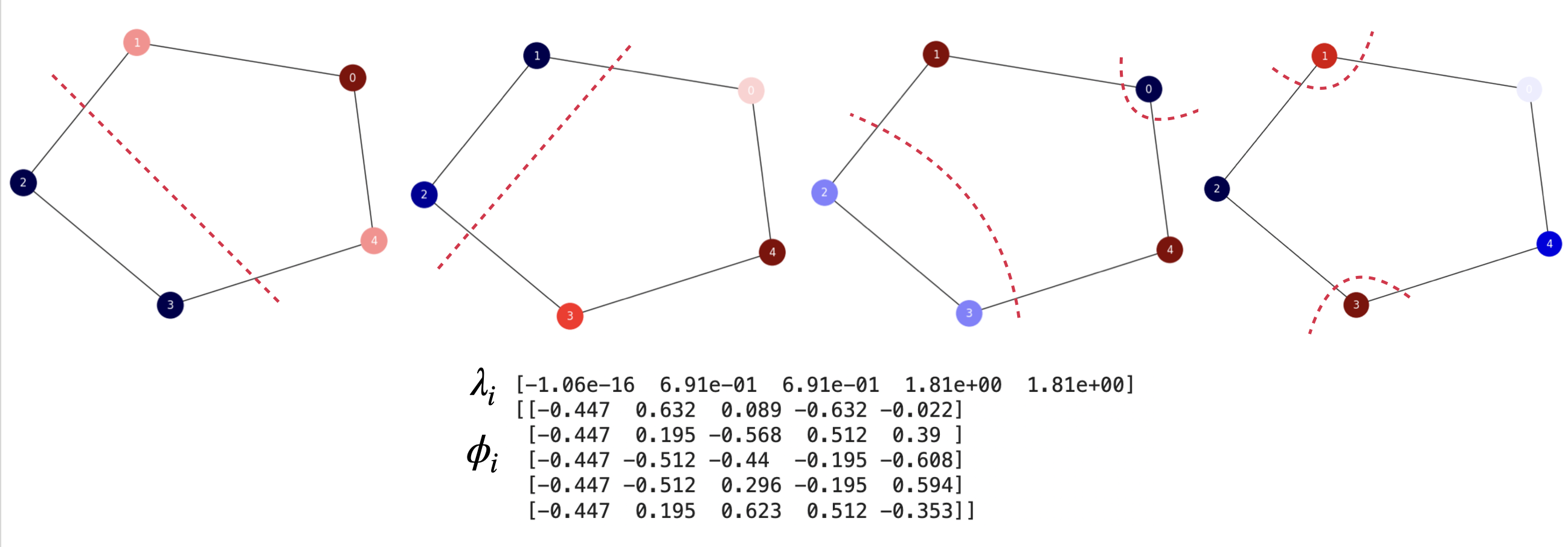
Fig. 7.4 \(C_5\). Normalized Laplacian’s spectrum and non-trivial eigenvectors.

7.1.2.1. The Cheeger constant

The Fiedler value \(\lambda_2\) is frequently used to quantify how weak is the graph (the smaller \(\lambda_2\) the weaker \(G\)). This is particularly interesting when bounding the so called Cheeger constant. We define it as follows:

Consider a partition \(V=A\cup \bar{A}\), \(A\cap \bar{A}=\emptyset\), then the conductance of the partition is

\[ h(A) = \frac{cut(A,\bar{A})}{\min\{|A|,|\bar{A}|\}}\;, \]

and the Cheeger constant is the *minimum conductance por any partition of \(V\) (defined as by subset \(A\subseteq V\) and its complementary \(\bar{A}=V-A\)):

\[ h_G = \min_{A\subseteq V}h(A)\;. \]

Since its seems that minimizing the Cheeger constant is quite similar to minimizing \(\text{Rcut}(A,\bar{A})\), it is not surprising that computing the Cheeger constant is NP-hard (we must evaluate all the possible \(2^{|V|}\) partitions/subsets of \(V\)). However, since we have the Fiedler value, which is \(\lambda_2>0\) for a connected graph, we have the following fundamental bound of spectral graph theory:

\[ 2h_G\ge \lambda_2\ge \frac{h_G^2}{2}\;. \]

The proof can be found in Chung’s book (Chapter~2). Anyway, this bound is interesting since it tells us how precise is the approximation of the Cheeger constant by using \(\lambda_2\) (also known as the spectral gap). The wider the bottleneck of the graph (large conductance) the worse the approximation.

7.1.2.2. The Mixing time

The spectral gap \(\lambda_2\) is also key to characterize the mixing time of a graph. Remember that the mixing time of a transition matrix \(\mathbf{P}\) associated with a graph \(G=(V,E)\) is the time needed to reach the steady state distribution \(\pi\) where the probability of going from a given node \(i\) to any other \(i\) is proportional to the degree of the destination: \(\pi_i=\frac{d_j}{\text{vol}(G)}\).

In order to explain the link between the spectral gap and the mixing time we follow some formal steps:

1. Link the matrices \(\mathbf{P}\) and \(\tilde{\mathbf{P}}\).

2. Link the eigenvectors of \(\mathbf{P}\) and \(\tilde{\mathbf{P}}\).

3. Apply the spectral theorem.

Link the matrices. The matrices \(\mathbf{P}=\mathbf{D}^{-1}\mathbf{A}\) and \(\tilde{\mathbf{P}}=\mathbf{D}^{-1/2}\mathbf{A}\mathbf{D}^{-1/2}\) are related as follows:

\[\begin{split} \begin{align} \tilde{\mathbf{P}}=\mathbf{D}^{-1/2}\mathbf{A}\mathbf{D}^{-1/2} &\Rightarrow \mathbf{D}^{-1/2}\tilde{\mathbf{P}}=\mathbf{D}^{-1/2}\mathbf{D}^{-1/2}\mathbf{A}\mathbf{D}^{-1/2}\\ &\Rightarrow \mathbf{D}^{-1/2}\tilde{\mathbf{P}}=\mathbf{D}^{-1}\mathbf{A}\mathbf{D}^{-1/2}\\ &\Rightarrow \mathbf{D}^{-1/2}\tilde{\mathbf{P}}\mathbf{D}^{1/2}=\mathbf{D}^{-1}\mathbf{A}\mathbf{D}^{-1/2}\mathbf{D}^{1/2}\\ &\Rightarrow \mathbf{D}^{-1/2}\tilde{\mathbf{P}}\mathbf{D}^{1/2}=\mathbf{D}^{-1}\mathbf{A}\\ &\Rightarrow \mathbf{D}^{-1/2}\tilde{\mathbf{P}}\mathbf{D}^{1/2}=\mathbf{P} \end{align} \end{split}\]

i.e. \( \mathbf{P} = \mathbf{D}^{-1/2}\tilde{\mathbf{P}}\mathbf{D}^{1/2}\;. \)

Link the eigenvectors. If \(\phi\) is an eigenvector of \(\mathbf{P}\) with eigenvalue \(\lambda\), then \(\tilde{\phi}=\mathbf{D}^{1/2}\phi\) is an eigenvector of \(\tilde{\mathbf{P}}\) with the same eigenvalue \(\lambda\):

\[\begin{split} \begin{align} \mathbf{P}\phi = \lambda\phi\; &\Rightarrow \mathbf{D}^{-1/2}\tilde{\mathbf{P}}\mathbf{D}^{1/2}\phi = \lambda\phi\\ &\Rightarrow \mathbf{D}^{1/2}\mathbf{D}^{-1/2}\tilde{\mathbf{P}}\mathbf{D}^{1/2}\phi = \lambda\mathbf{D}^{1/2}\phi\\ &\Rightarrow \tilde{\mathbf{P}}\mathbf{D}^{1/2}\phi = \lambda\mathbf{D}^{1/2}\phi\\ &\Rightarrow \tilde{\mathbf{P}}\tilde{\phi} = \lambda\tilde{\phi}\\ \end{align} \end{split}\]

Apply the spectral theorem. Firstly, we apply the spectral theorem to \(\tilde{\mathbf{P}}\):

\[ \tilde{\mathbf{P}}=\sum_{i=1}^{n}\lambda_i\tilde{\phi}_i\tilde{\phi}_i^T\;, \]

Then, following Lovasz’s Random Walks on Graphs: A Survey we plug the above expansion in \(\mathbf{P} = \mathbf{D}^{-1/2}\tilde{\mathbf{P}}\mathbf{D}^{1/2}\):

\[ \mathbf{P} = \mathbf{D}^{-1/2}\tilde{\mathbf{P}}\mathbf{D}^{1/2} = \sum_{i=1}^n\lambda_i\mathbf{D}^{-1/2}\tilde{\phi}_i\tilde{\phi}_i^T\mathbf{D}^{1/2}\;. \]

Now, we expand the above expression as follows:

\[ \mathbf{P} = \lambda_1\mathbf{D}^{-1/2}\tilde{\phi}_1\tilde{\phi}_1^T\mathbf{D}^{1/2} + \sum_{i=2}^n\lambda_i\mathbf{D}^{-1/2}\tilde{\phi}_i\tilde{\phi}_i^T\mathbf{D}^{1/2}\;. \]

Since \(\lambda_1=1\) and \(\tilde{\phi}_1=\mathbf{D}^{1/2}\mathbf{1}\), the first term of the above expression becomes:

\[\begin{split} \begin{align} 1\cdot\mathbf{D}^{-1/2}\tilde{\phi}_1\tilde{\phi}_1^T\mathbf{D}^{1/2} &= \mathbf{D}^{-1/2}\mathbf{D}^{1/2}\mathbf{1}(\mathbf{D}^{1/2}\mathbf{1})^T\mathbf{D}^{1/2}\\ &= \mathbf{1}\mathbf{1}^T\mathbf{D}^{1/2}\mathbf{D}^{1/2}\\ &= \mathbf{1}\mathbf{1}^T\mathbf{D}\\ &= \mathbf{1}\mathbf{1}^T\mathbf{D}\\ \end{align} \end{split}\]

where we define \(\mathbf{Q}=\mathbf{1}\mathbf{1}^T\mathbf{D}\) is a matrix whose all rows are repeated and they are equal to

\[ \mathbf{Q}_{i:}=[d_1\; d_2\; \ldots\; d_n]\;, \]

Remember (from the previous topic) that

\[ \lim_{t\rightarrow\infty}\mathbf{P}^t = \Pi\; \]

where

\[ \Pi_{i:} = \pi = [\frac{d_1}{\text{vol}(G)}\; \frac{d_2}{\text{vol}(G)}\;\ldots\; \frac{d_n}{\text{vol}(G)}\;]\;, \]

i.e. all the stationary distribution is repeated in each row of \(\Pi\).

As a result, \(\Pi\) is just a normalized version of \(\mathbf{Q}\), i.e. we may interpret \(\mathbf{Q}_{i:}\) as an unnormalized degree distribution. This is exactly all we need for the proof since we have:

\[\begin{split} \begin{align} \mathbf{P} &= \mathbf{Q} + \sum_{i=2}^n\lambda_i\mathbf{D}^{-1/2}\tilde{\phi}_i\tilde{\phi}_i^T\mathbf{D}^{1/2} \\ &\approx \Pi + \sum_{i=2}^n\lambda_i\mathbf{D}^{-1/2}\tilde{\phi}_i\tilde{\phi}_i^T\mathbf{D}^{1/2}\\ &\approx \Pi + \sum_{i=2}^n\lambda_i\mathbf{D}^{-1/2}\mathbf{R}_i\mathbf{D}^{1/2}\;, \end{align} \end{split}\]

Now, each term \(\tilde{\phi}_i\tilde{\phi}_i^T\) is an \(n\times n\) matrix \(\mathbf{R}_i\) where \(\mathbf{R}_i(u,v)=\tilde{\phi}_i(u)\tilde{\phi}_i(v)\).

As a result, taking the components \(p_{uv}\) of \(\mathbf{P}\), we have:

\[ p_{uv} \approx \pi_{uv} + \sum_{i=2}^n\lambda_i\tilde{\phi}_i(u)\tilde{\phi}_i(v)\sqrt{\frac{d_v}{d_u}}\;. \]

Finally, applying the spectral problem to the power \(\mathbf{P}^t\) we have

\[ \mathbf{P}^t=\sum_{i=1}^{n}\lambda_i^t\phi_i\phi_i^T\;, \]

i.e. any matricial function (e.g the power, exponential, logartithn) is transferred to the spectrum!

Using this result, we have that

\[ p_{uv}^t \approx \pi_{uv} + \sum_{i=2}^n\lambda_i^t\tilde{\phi}_i(u)\tilde{\phi}_i(v)\sqrt{\frac{d_v}{d_u}}\;. \]

Which leads to

\[ p^t(v) \approx \pi(v) + \sum_{i=2}^n\lambda_i\tilde{\phi}_i(u)\tilde{\phi}_i(v)\sqrt{\frac{d_v}{d_u}}\;. \]

Then, the rate of convergence of \(\mathbf{P}\) to \(\Pi\) is given by

\[\begin{split} \begin{align} p^t(v) - \pi(v) &\approx \sum_{i=2}^n\lambda_i\tilde{\phi}_i(u)\tilde{\phi}_i(v)\sqrt{\frac{d_v}{d_u}}\\ |p^t(v) - \pi(v)| &\approx \left|\sum_{i=2}^n\lambda_i\tilde{\phi}_i(u)\tilde{\phi}_i(v)\sqrt{\frac{d_v}{d_u}}\right|\\ &< |\lambda_2^t|\left|\sum_{i=2}^n\tilde{\phi}_i(u)\tilde{\phi}_i(v)\sqrt{\frac{d_v}{d_u}}\right|\\ &< |\lambda_2^t|\cdot\sqrt{\frac{d_v}{d_u}}\;. \end{align} \end{split}\]

where the last simplification is due to the fact that \(\sum_{i=2}^n\tilde{\phi}_i(u)\tilde{\phi}_i(v)\le 1\) since the eigenvectors are orthonormal: \(\tilde{\Phi}\tilde{\Phi}^T=\mathbf{I}\).

Then, the rate of convergence to the steady distribution is fast if the spectral gap is small!

7.2. Commute Times and Embedding

7.2.1. Where do data live?

Consider a set of \(n\) points \(X=\{\mathbf{x}_1,\mathbf{x}_2,\ldots,\mathbf{x}_n\}\), with \(x_i\in 3D\). The natural metric in \(3D\) is the Euclidean distance \(\|\mathbf{x}_i - \mathbf{x}_j\|=\sqrt{\sum_{k=1}^3(\mathbf{x}_i(k)-\mathbf{x}_j(k))^2}\). See for instance the point cloud in Fig. 7.5.

Such a point cloud (called Swiss roll) is the typical representation of data such as images in low-dimensional spaces (one point per image) called manifolds. It is well known that these spaces have a curved geometry. Similar images, for instance are pretty close in a low-dimensional space but the semantic of such a similarity is barely consistent with the near-spherical clusters of Euclidean spaces.

As a result, when we try to cluster these data, which live in a curved-space, using Euclidean distances (see Fig. 7.5-left where we set \(C=3\) clusters), points far away in the curved manifold are clustered together.

Alternatively, we follow the approach proposed in the seminal paper of Tenenbaum et al.:

1. We create a graph \(G=(V,E)\) with \(|V|=n\), where there is an edge \(e=(i,j)\) if \(j\) is one of the \(K=10\) closest neighbors of \(i\). This is called a KNN graph or Nearest Neighbors graph. Well, the Euclidean distances \(\|\mathbf{x}_i - \mathbf{x}_j\|\) are only used to build the KNN graph.

2. After creating the KNN graph, we compute the three eigenvectors \(\phi_2\),\(\phi_3\) and \(\phi_4\) corresonding with the three non-trivial smallest eigenvalues \(\lambda_2\), \(\lambda_3\) and \(\lambda_4\) of the Laplacian.

3. It is well known that the encoding (also called embedding) of each \(\mathbf{x}_i\) as

\[ \mathbf{z}_i = [\phi_2(i)\;\phi_3(i)\; \phi_4(i)]^T \]

minimizes the ratio-cut loss of the KNN graph \(G=(V,E)\). As a result, when using Euclidean distance \(\|\mathbf{z}_i-\mathbf{z}_j\|\) in the transformed or latent space, we achieve a clustering consistent with the curved space (see Fig. 7.5-right).

In other words, as we have explained in the previous topic spectral partition leads to cluster the data in a way that is consistent with the curved geometry of the graph.

But, how do we know this? Because Tenembaum et al. found that the distances \(\|\mathbf{z}_i-\mathbf{z}_j\|\) are statistically correlated with the shortest path distances SP between the nodes, found by the Dijkstra or \(A^{\ast}\) algorithms!

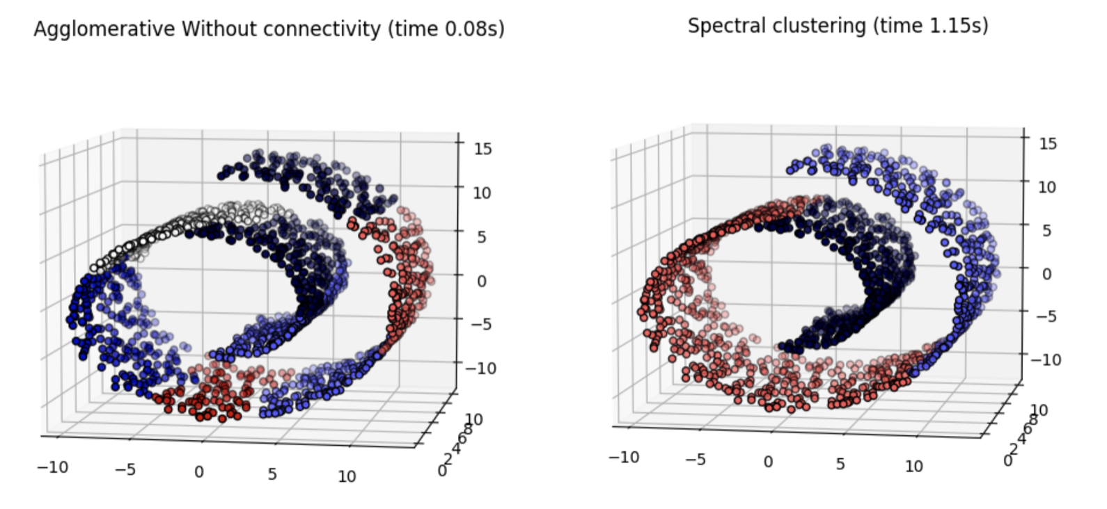
Fig. 7.5 Swiss-roll point cloud clustered using Euclidean distances (left) vs clustered using Spectral theory (right).

However, we know that shortest path SP distance are not strictly respectful with the structure of the graph. For instance, in an SBM with an important bottleneck, we may have two nodes pretty close either when they are in the same community or in different communities, but this fact is not reflected by SP distance.

As a result, we have used hitting and commute times in the practical lessons of this subject. These “times” are really distances which are compliant with the curved geometry of graphs and they can be efficiently approximated via spectral theory.

7.2.2. Commute Times and Spectral Gap

The commute time \(CT(u,v)=H(u,v)+H(v,u)\) between two nodes \(u\) and \(v\) is the expected time needed by a random walk departing from \(u\) to reach \(v\) (hitting time \(H(u,v)\)) and come back (hit \(u\) from \(v\), \(H(v,u)\)).

As we know from the practical lessons, commute times are related with the relative size of the bottleneck (or Cheeger constant) which is estimated by the spectral gap. If the bottleneck/spectral gap is small, random walk take a lot of time to travel from one community to another (see Fig. 7.6).

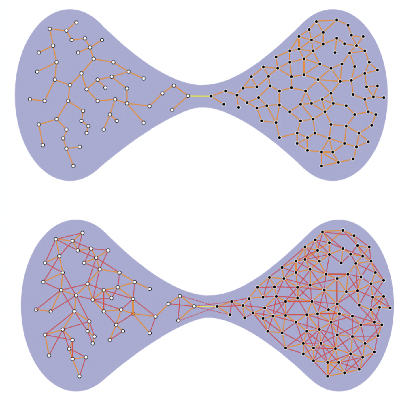
Fig. 7.6 Commute Times (CT) and spectral gap. Top: small spectral gap gives large CTs. Bottom: larger spectral gap gives smaller CTs. Source: Francisco Escolano in the Pattern Recognition Journal

The Lovasz Bound. As we will see below, a small spectral gap is essential to obtain informative CTs. In other words, if the spectral gap is not small, the commute time can be approximated as follows

\[ CT(u,v)\approx \frac{1}{d_u} + \frac{1}{d_v}\;. \]

This was a key observation by von Luxburg et al. based in a bound proposed by Lovasz. This bound, illustrated in Fig. 7.7 simply says that: the smaller the spectral gap the more different are the CT from \(\frac{1}{d_u} + \frac{1}{d_v}\).

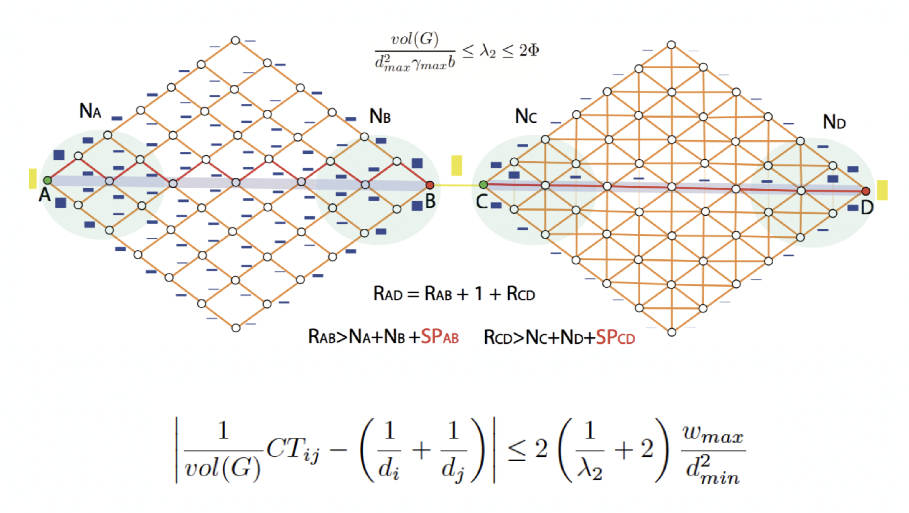
Fig. 7.7 Illustration of the Lovasz bound. Source: Francisco Escolano in the Pattern Recognition Journal

A priori, this is a very simple conclusion but it has deep implications. Commute Times are not informative in large KNN graphs, large Erdos-Renyi graphs among other graphs with large spectral gap (close to \(1\)) studied in the previous section.

One way of making the CTs informative is to rewire the graph while keeping the spectral gap as smallest as possible. For instance, in Fig. 7.7 we can see than the right community is denser than the left one and this reduces the spectral gap!

7.2.3. Spectral Commute Times

For the spectral version of commute times, we rely on the Green’s function as it is done in the yet classic paper of my mentor Edwin Hancock:

Green’s function. A key matrix to compute both the hitting and commute times is the so called Green’s function \(G\) or pseudoinverse \(\triangle^{+}\) of the Laplacian \(\triangle\). For a connected graph, we have the following component-wise equation

\[ G(u,v) = \sum_{i=2}^{|V|}\frac{1}{\lambda_i}\phi_i(u)\phi_i(v)\; \]

Hitting time. \(H(u,v)\) is spectrally determined by

\[\begin{split} \begin{align} H(u,v) &= \text{vol}(G)\left[G(v,v) - G(u,v)\right]\\ &= \text{vol}(G)\left[\sum_{i=2}^{|V|}\frac{1}{\lambda_i}\phi_i(v)^2\ - \sum_{i=2}^{|V|}\frac{1}{\lambda_i}\phi_i(u)\phi_i(v)\right]\\ &= \text{vol}(G)\sum_{i=2}^{|V|}\frac{1}{\lambda_i}\left[\phi_i(v)^2-\phi_i(u)\phi_i(v)\right]\\ &= \text{vol}(G)\frac{1}{\lambda_2}\left[\phi_2(v)^2-\phi_2(u)\phi_2(v)\right] + \ldots + \text{vol}(G)\frac{1}{\lambda_n}\left[\phi_n(v)^2-\phi_n(u)\phi_n(v)\right]\;. \end{align} \end{split}\]

Since \(\lambda_2\le\lambda_3\le\ldots\le\lambda_n\), the importance of each term in the sum is inversely proportional to the corresponding \(\lambda_i\). This means that if \(\lambda_2\rightarrow 0\) (very small spectral gap), we have:

\[ H(u,v)\approx \text{vol}(G)\left[\phi_2(v)^2-\phi_2(u)\phi_2(v)\right]\;. \]

Reminder. It is key to note that in general \(H(u,v)\neq H(v,u)\).

Commute time. \(CT(u,v)=H(u,v) + H(v,u)\) is spectrally determined by the spectral computations of \(H(u,v)\) and \(H(v,u)\):

\[\begin{split} \begin{align} \frac{CT(u,v)}{\text{vol}(G)} &= H(u,v) + H(v,u)\\ &= G(v,v) - G(u,v) + G(u,u) - G(v,u)\\ &= G(u,u) + G(v,v) - 2G(u,v)\;. \end{align} \end{split}\]

Commute times are metrics. Then, \(CT(u,v)=\text{vol}(G)\left[G(u,u) + G(v,v) - 2G(u,v)\right]\) because the Green’s function is commutative \(G(u,v)=G(v,u)\). As a result, \(CT(u,v)\) is formally a distance between two nodes.

Then, the spectral computation of the commute time can be derived easily and results in

\[ CT(u,v) = \text{vol}(G)\sum_{i=2}^{|V|}\frac{1}{\lambda_i}\left[\phi_i(u)-\phi_i(v)\right]^2\;. \]

Again, if \(\lambda_2\rightarrow 0\), we have:

\[ CT(u,v) = \text{vol}(G)\frac{1}{\lambda_2}\left[\phi_2(u)-\phi_2(v)\right]^2\;. \]

It is not surpising to see that the commute time between nodes in a graph changes according to the structure of the graph. See the exercise below.

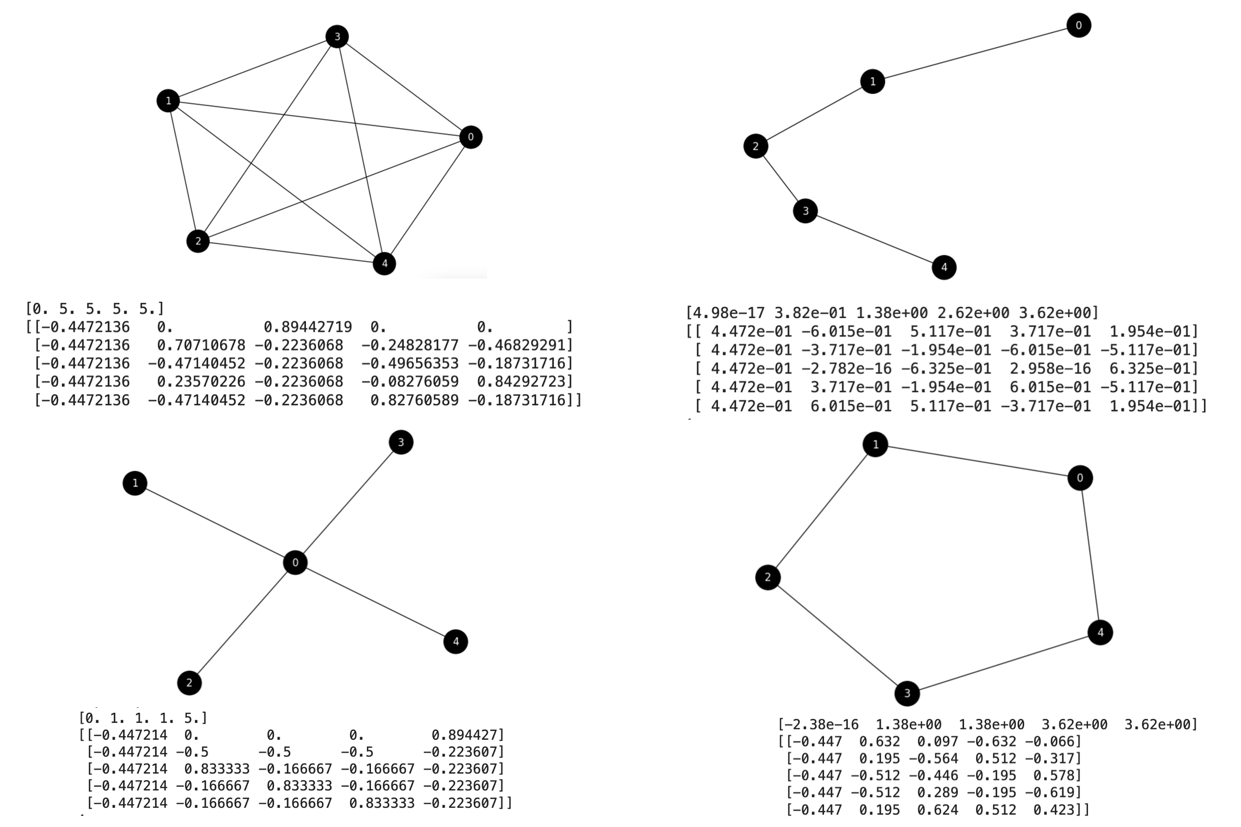
Fig. 7.8 Spectra and eigenvalues of the unnormalized Laplacian of several basic graphs.

Exercise. Consider graphs Fig. 7.8. Suppose that we only have the spectral gap and the Fiedler vector of the Laplacian specified in the figure.

Then, approximate the commute times between nodes \(0\) and \(4\) in the four graphs: \(K_5\), \(S_5\), \(P_5\) and \(C_5\) in the figure. Note that instead of using the spectra and eigenvalues of the normalized Laplacian, herein we use those of the unnormalized one! Use only \(\lambda_2\) and \(\phi_2\) and comment the meaning of the result: is it consistent with theory? How it is related with the approximate value \(CT(u,v)=\frac{1}{d_u} + \frac{1}{d_v}\). Take two decimals.

Complete graph. We have that the volume of this graph is \(\text{vol}(G)=5\cdot 4 = 20\) and \(\lambda_2=5\). Then

\( \begin{align} CT(0,4) &= \text{vol}(G)\frac{1}{\lambda_2}\left[\phi_2(u)-\phi_2(v)\right]^2\\ &= 20\cdot\frac{1}{5}\left[\phi_2(0)-\phi_2(4)\right]^2 = 20\cdot\frac{1}{5}\left[0-(-0.47)\right]^2\\ &= 20\cdot\frac{1}{5}\cdot 0.22 = 0.88\\ \end{align} \)

Star graph. We have that the volume of this graph is \(\text{vol}(G)=4 + 4 = 8\) and \(\lambda_2=1\). Then

\( \begin{align} CT(0,4) &= \text{vol}(G)\frac{1}{\lambda_2}\left[\phi_2(u)-\phi_2(v)\right]^2\\ &= 8\cdot\frac{1}{1}\left[\phi_2(0)-\phi_2(4)\right]^2 = 8\cdot\frac{1}{1}\left[0-(-0.16)\right]^2\\ &= 8\cdot\frac{1}{1}\cdot 0.02 = 0.16\\ \end{align} \)

Path graph. We have that the volume of this graph is \(\text{vol}(G)=1 + 2 + 2 + 2 + 1 = 8\) and \(\lambda_2=0.38\). Then

\( \begin{align} CT(0,4) &= \text{vol}(G)\frac{1}{\lambda_2}\left[\phi_2(u)-\phi_2(v)\right]^2\\ &= 8\cdot\frac{1}{0.38}\left[\phi_2(0)-\phi_2(4)\right]^2 = 8\cdot\frac{1}{0.38}\left[0-0.6)\right]^2\\ &= 8\cdot\frac{1}{0.38}\cdot 0.36 = 7.57\\ \end{align} \)

Cycle graph. We have that the volume of this graph is \(\text{vol}(G)=5\cdot 2 = 10\) and \(\lambda_2=0.13\). Then

\( \begin{align} CT(0,4) &= \text{vol}(G)\frac{1}{\lambda_2}\left[\phi_2(u)-\phi_2(v)\right]^2\\ &= 10\cdot\frac{1}{0.13}\left[\phi_2(0)-\phi_2(4)\right]^2 = 10\cdot\frac{1}{0.13}\left[0.63-0.19)\right]^2\\ &= 10\cdot\frac{1}{0.13}\cdot 0.19 = 14.6\\ \end{align} \)

Comments. We have the following CTs between nodes \(0\) and \(4\) in the different graphs:

\( \begin{align} & K_5:\;\; CT(0,4)=0.88\\ & S_5:\;\; CT(0,4)=0.16\\ & P_5:\;\; CT(0,4)=7.57\\ & C_5:\;\; CT(0,4)=14.6\\ \end{align} \)

Complete graphs are characterized by having the same CT between any pair of nodes. This value is small \(CT(0,4)=0.88\) because random walks have a uniform probability \(\frac{1}{n-1}\) of reaching each of the nodes in a single step. The approximate CT is

\( CT(0,4)\approx\frac{1}{d_0} + \frac{1}{d_4}=\frac{1}{n-1} + \frac{1}{n-1} = 2\frac{1}{n-1} = 2\frac{1}{4} = 0.5\;. \)

Star graphs are characterized by having the same CT between the center node \(0\) and the remaining one (for instance \(4\)). This value is smaller than that of the complete graph \(CT(0,4)=0.16\) because random walks have a uniform probability \(\frac{1}{n-1}\) of reaching each of the non central nodes in a single step (as in the complete graph). However, non-central nodes have a unit probability of reaching the center node (remember than hitting times are assymetric in general). The approximate CT is

\( CT(0,4)\approx\frac{1}{d_0} + \frac{1}{d_4}=\frac{1}{n-1} + 1 = \frac{n-1+1}{n-1} = \frac{n}{n-1}=\frac{5}{4} = 1.25\;. \)

This is clearly an over-estimation because the Fiedler value for this graph is smaller to that of the complete graph.

Path graphs are characterized by having large CT for distant nodes. This is due to the fact that the path graph is formally a tree, i.e. it does not have loops. As a result, the CT between a pair of nodes in this graph is proportional to the shortest path (SP) distance between the nodes. In this case, we have \(CT(0,4)=7.57\approx 2\cdot 3=6\). The approximate CT is

\( CT(0,4)\approx\frac{1}{d_0} + \frac{1}{d_4}= 1 + 1 = 2\;. \)

This is clearly an under-estimation because the Fiedler value for this graph is smaller those of the complete graph and the star graph.

Cycle graphs are characterized by having large CT for distant nodes. Observe that the probability of leaving a node is always \(1/2\), but we may return back with the same probability. Therefore, for reaching node \(4\) from \(0\), we may either go through the nodes \(1\), \(2\) and \(3\) or to go directly to \(4\). This leads to the largest CT in these analyzed graphs: \(CT(0,4)=14.6\). The approximate CT is

\( CT(0,4)\approx\frac{1}{d_0} + \frac{1}{d_4}= \frac{1}{2} + \frac{1}{2} = 1\;. \)

This is clearly an under-estimation because the Fiedler value for this graph is between that of the star graph and that of the complete graph.

7.2.4. Commute-Times Embedding

As we have seen before, when studying where do data live, embedding the nodes of a graph consists of finding a vector representation of each node \(\mathbf{z}_u,\;u\in V\) where the Euclidean distance \(\|\mathbf{z}_u-\mathbf{z}_v\|\) is consistent with the structural distance between the nodes \(u\) and \(v\) in the graph.

In the original paper of Tenenbaum et al., we have that making

\[ \mathbf{z}_u = [\phi_2(u)\;\phi_3(u)\; \phi_4(u)\;\ldots\; \phi_n(u)]^T \]

implies that \(\|\mathbf{z}_u-\mathbf{z}_v\|\) is statistically correlated with the shortest path distances SP between the nodes. This fact was key to found correlations between the info in the eigenvectors and more interesting structural distances such as the commute times.

Since the commute times is by definition a distance, it is trivial to check that the columns of this matrix

\[ \mathbf{Z} = \sqrt{\text{vol}(G)}\mathbf{\Lambda}^{-1/2}\Phi^T\;\Rightarrow CT(u,v) = \|\mathbf{z}_u-\mathbf{z}_v\|^2\;. \]

The proof is as follows:

• Matrix \(\mathbf{Z}\) has originally dimension \(n\times n\) and the embedding \(\mathbf{z}_u\) of node \(u\) is in the column \(u\).

• Let us see the structure of a row \(k\), which encodes the \(k-\)th dimension of the embedding \(\mathbf{z}_u\).

\[ \mathbf{Z}_{k:} = \mathbf{\Lambda}^{-1/2}\left[\phi_1(u)\;\phi_2(u)\; \phi_3(u)\;\ldots\; \phi_n(u)\right]\;, \]

where \(\Phi\) is the matrix of eigenvectors (columns from the smallest to the largest eigenvectors) and \(\Lambda=\text{diag}(\lambda_1\;\lambda_2\;\ldots\;\lambda_n)\) is the diagonal matrix with the spectrum of the Laplacian in the diagonal.

Then, discarding the \(\sqrt{\text{vol}(G)}\) for a while we have

\[ \mathbf{Z}_{k:} = \left[\frac{\phi_k(1)}{\sqrt{\lambda_k}}\;\frac{\phi_k(2)}{\sqrt{\lambda_k}}\; \frac{\phi_k(3)}{\sqrt{\lambda_k}}\;\ldots\; \frac{\phi_k(n)}{\sqrt{\lambda_k}}\right]\;. \]

• Actually the first row is normalized by \(\lambda_1=0\) and we assume that this row is:

\[ \mathbf{Z}_{1:} = \left[\frac{\phi_1(1)}{\sqrt{\lambda_1}}\;\frac{\phi_1(2)}{\sqrt{\lambda_1}}\; \frac{\phi_1(3)}{\sqrt{\lambda_1}}\;\ldots\; \frac{\phi_1(n)}{\sqrt{\lambda_1}}\right] = \left[0\; 0\; 0\;\ldots\; 0\right]\;. \]

• There are as many rows as dimensions of the embedding and the first dimension is always zero valued. This means that all the embeddings are centered.

• Consider for instance that we have only the information of the Fiedler vector. Then, we have only two rows (the first one which all zeros and the second one). If we discard the first dimension we have (after incorporating the term \(\sqrt{\text{vol}(G)}\)):

\[ \mathbf{Z}_{2:} = \sqrt{\text{vol}(G)}\left[\frac{\phi_2(1)}{\sqrt{\lambda_2}}\;\frac{\phi_2(2)}{\sqrt{\lambda_2}}\; \frac{\phi_2(3)}{\sqrt{\lambda_2}}\;\ldots\; \frac{\phi_2(n)}{\sqrt{\lambda_2}}\right] = \left[\mathbf{z}_1\; \mathbf{z}_2\; \mathbf{z}_3\;\ldots\; \mathbf{z}_n\right]\;.\;. \]

and obviously incorporating

\[ \|\mathbf{z}_u-\mathbf{z}_v\| = \text{vol}(G)\left[\frac{\phi_2(u)}{\sqrt{\lambda_2}} - \frac{\phi_2(v)}{\sqrt{\lambda_2}}\right]^2 = \text{vol}(G)\frac{1}{\lambda_2}\left[\phi_2(u) - \phi_2(v)\right]^2\approx CT(u,v)\;. \]

and similarly for \(d\) dimensions, where the commute time is exact if \(d\rightarrow n\). More generally

\[ \|\mathbf{z}_u-\mathbf{z}_v\| = \text{vol}(G)\sum_{k=2}^d\left[\frac{\phi_k(u)}{\sqrt{\lambda_k}} - \frac{\phi_k(v)}{\sqrt{\lambda_k}}\right]^2 = \text{vol}(G)\sum_{k=2}^d\frac{1}{\lambda_k}\left[\phi_k(u) - \phi_k(v)\right]^2\approx CT(u,v)\;. \]

The convergence to the optimal number of dimensions is faster when the spectral gap is very small!

Exercise. Back to the graphs in Fig. 7.8. Compute the CT embeddings of nodes \(0\) and \(4\) in each graph. Consider two dimensions (in addition to the zero) and take two decimals. Plot the \(2D\) of all the nodes in the plane and comment on the results.

Complete graph. We have that the volume of this graph is \(\text{vol}(G)=5\cdot 4 = 20\) and \(\lambda_2=\lambda_3=5\). Then

\( \begin{align} \mathbf{Z}_{2:} &= \text{vol}(G)\left[\frac{\phi_2(1)}{\sqrt{5}}\;\frac{\phi_2(2)}{\sqrt{5}}\;\ldots\; \frac{\phi_2(5)}{\sqrt{5}}\right] = \frac{20}{\sqrt{5}}\cdot\left[+0.00\; +0.70\; -0.47\; +0.23\; -0.47\right]\\ \mathbf{Z}_{3:} &= \text{vol}(G)\left[\frac{\phi_3(1)}{\sqrt{5}}\;\frac{\phi_3(2)}{\sqrt{5}}\;\ldots\; \frac{\phi_3(5)}{\sqrt{5}}\right] = \frac{20}{\sqrt{5}}\cdot\left[+0.89\; -0.22\; -0.22\; -0.22\; -0.22\right]\\ \end{align} \)

See that the \(2D\) embedding of nodes \(3\) and \(5\) (\(2\) and \(4\) in Fig. 7.9) have the same embedding, i.e. they collide.

Star graph. We have that the volume of this graph is \(\text{vol}(G)=4 + 4 = 8\) and \(\lambda_2=\lambda_3=1\). Then

\( \begin{align} \mathbf{Z}_{2:} &= \text{vol}(G)\left[\frac{\phi_2(1)}{\sqrt{1}}\;\frac{\phi_2(2)}{\sqrt{1}}\;\ldots\; \frac{\phi_2(5)}{\sqrt{1}}\right] = \frac{8}{\sqrt{1}}\cdot\left[+0.00\; -0.50\; +0.83\; -0.16\; -0.16\right]\\ \mathbf{Z}_{3:} &= \text{vol}(G)\left[\frac{\phi_3(1)}{\sqrt{1}}\;\frac{\phi_3(2)}{\sqrt{1}}\;\ldots\; \frac{\phi_3(5)}{\sqrt{1}}\right] = \frac{8}{\sqrt{5}}\cdot\left[+0.00\; -0.50\; -0.16\; +0.83\; -0.16\right]\\ \end{align} \)

See that in the \(2D\) embedding, node \(5\) (\(4\) in Fig. 7.9) is closer to node \(1\) (\(0\) in the figure) than others.

Path graph. We have that the volume of this graph is \(\text{vol}(G)=1 + 2 + 2 + 2 + 1 = 8\) and \(\lambda_2=0.38\), \(\lambda_3=1.38\). Then

\( \begin{align} \mathbf{Z}_{2:} &= \text{vol}(G)\left[\frac{\phi_2(1)}{\sqrt{0.38}}\;\frac{\phi_2(2)}{\sqrt{0.38}}\;\ldots\; \frac{\phi_2(5)}{\sqrt{0.38}}\right] = \frac{8}{\sqrt{0.38}}\cdot\left[-0.60\; -0.37\; -0.27\; +0.37\; +0.60\right]\\ \mathbf{Z}_{3:} &= \text{vol}(G)\left[\frac{\phi_3(1)}{\sqrt{1.38}}\;\frac{\phi_3(2)}{\sqrt{1.38}}\;\ldots\; \frac{\phi_3(5)}{\sqrt{1.38}}\right] = \frac{8}{\sqrt{1.38}}\cdot\left[+0.51\; -0.19\; -0.63\; -0.19\; +0.51\right]\\ \end{align} \)

See that the \(2D\) embedding in Fig. 7.9 is even more symmetric than the provided by Networkx’s “spring layout”. This is because the eigenvalues are different and add more flexibility to the drawing. However, what is essential here is that the eigenvectors capture well the symmetries of the graph.


Cycle graph. We have that the volume of this graph is \(\text{vol}(G)=5\cdot 2 = 10\) and \(\lambda_2=\lambda_3=1.38\). Then

\( \begin{align} \mathbf{Z}_{2:} &= \text{vol}(G)\left[\frac{\phi_2(1)}{\sqrt{1.38}}\;\frac{\phi_2(2)}{\sqrt{1.38}}\;\ldots\; \frac{\phi_2(5)}{\sqrt{1.38}}\right] = \frac{10}{\sqrt{1.38}}\cdot\left[+0.63\; +0.19\; -0.51\; -0.51\; -0.19\right]\\ \mathbf{Z}_{3:} &= \text{vol}(G)\left[\frac{\phi_3(1)}{\sqrt{1.38}}\;\frac{\phi_3(2)}{\sqrt{1.38}}\;\ldots\; \frac{\phi_3(5)}{\sqrt{1.38}}\right] = \frac{10}{\sqrt{1.38}}\cdot\left[+0.09\; -0.56\; -0.44\; +0.28\; +0.62\right]\\ \end{align} \)

See that the \(2D\) embedding in Fig. 7.9 is quite similar to the provided by Networkx’s “spring layout”, even when the second and third eigenvalues are similar. This is because the eigenvectors capture well the symmetries in the graph.

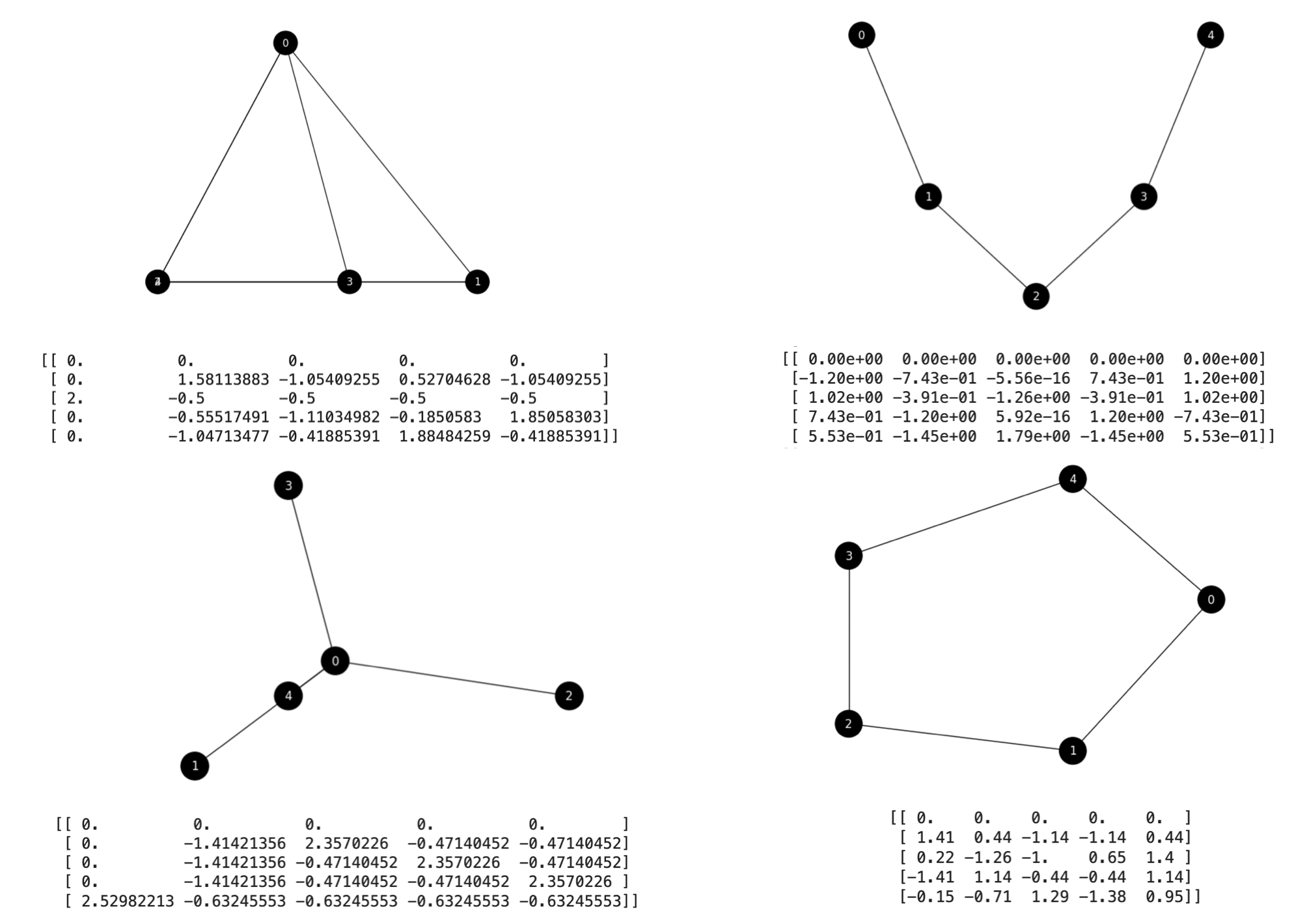
Fig. 7.9 Reconstruction of the basic graphs from their Commute-Times Embeddings.

Solutions. The resulting Commute-Times embeddings are plotted in Fig. 7.9 where we also plot the graphs taken from the second and third dimensions of each node. Note that for the complete graph, nodes \(2\) and \(4\) collide. For the star graph node \(4\) is misplaced. However for the path graph and the cycle graph the reconstructed graph fits perfectly the “spring layout” of Networkx. This good results for the path and cycle graphs do not have notable nodes with higher degrees than others. Nodes with large degree tend to distort the embedding even when the graph has structural symmetries.

Just to finish this topic with a link with real data and the practices, we plot the commute-times embeddings of the well-known Cora dataset in Fig. 7.10. The top-right is the embedding of the second and third eigenvectors and it is barely informative. The bottom-right however includes the fourth eigenvector and a more advanced (TSNE) projection.

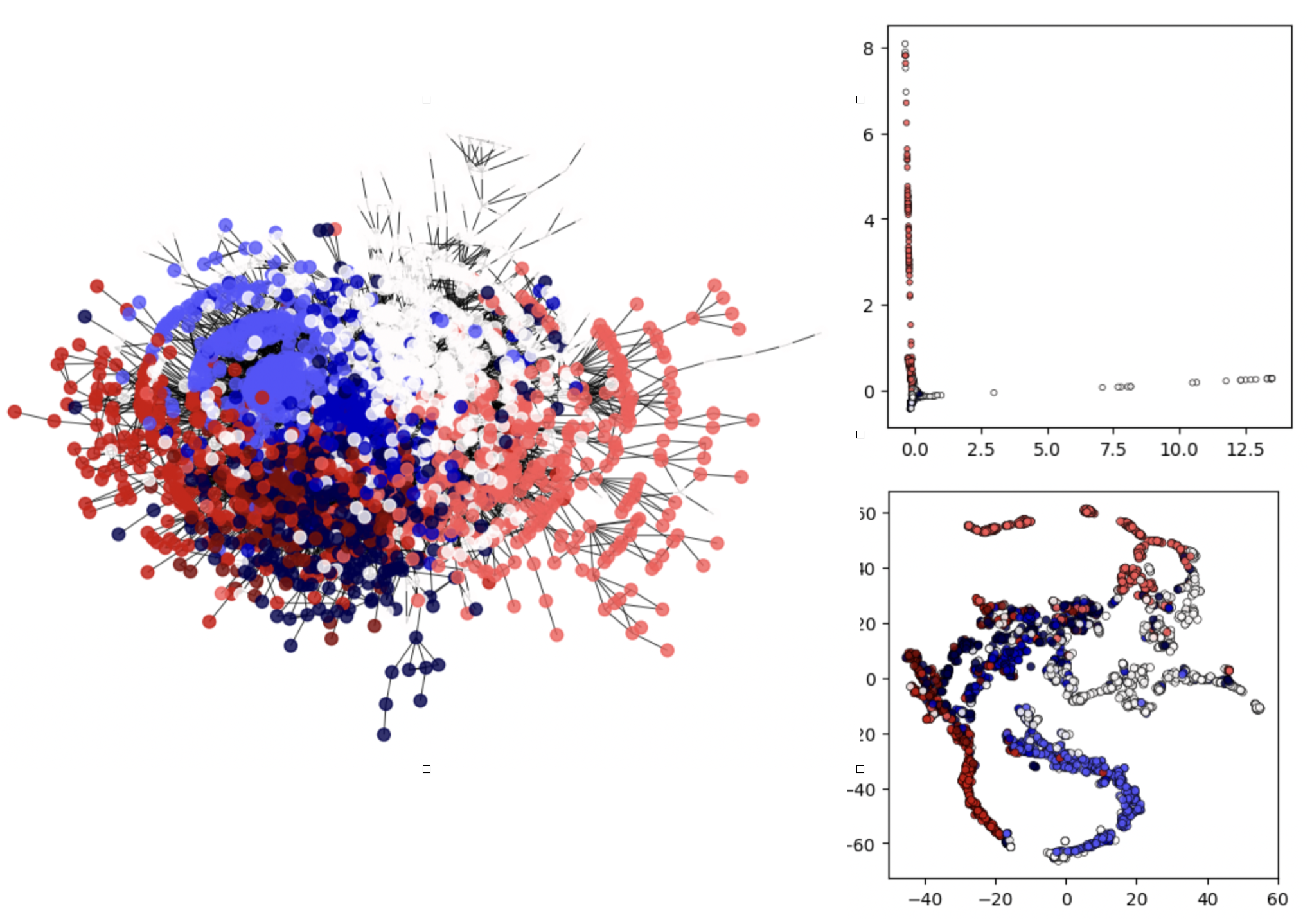
Fig. 7.10 Cora dataset: Commute-Times Embeddings.