2. Combinatorics as counting#
Our Discrete Brain must be able of counting objects, i.e. it must be answer questions such as:
How many subsets are in a set of size \(n\)?
How many subsets of \(k\) elements are in a set of size \(n\)?
How many injective functions can map two sets \(A\) and \(B\) with sizes \(m\) and \(n\)?
The above questions are referred to as counting tasks, insofar they can be decomposed into simpler tasks. Consider for instance the last task. We have two sets \(A\) and \(B\) with sizes \(m\) and \(n\), where \(m\le n\). Then:
We are considering injective (one-to-one) functions \(f:X\rightarrow Y\), i.e. the reference is \(X\) (we reason from left to right).
In each function \(f\), each element \(x_i\in X\) must mapped either to one and only only one element \(y_j\in Y\) or to none of them.
For instance, in setfunction we have \(X=\{a,b,c\}\) and \(Y=\{1,2,3,4\}\), i.e \(m=3\) and \(n=4\). The mapping, say \(f\), is injective since: (a) every element in \(X\) has an image and only one image in \(Y\), (b) no elements in \(Y\) is the image of more than one element in \(X\).
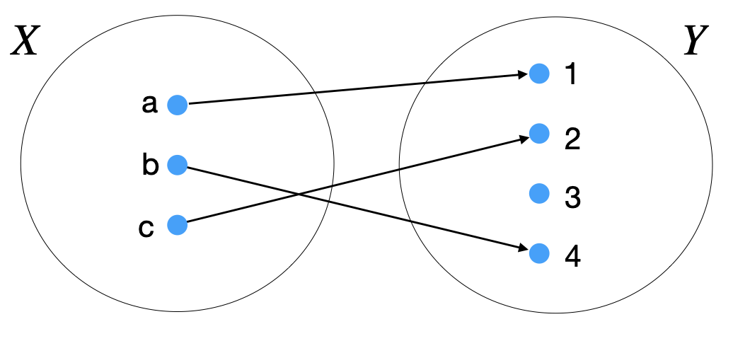
Fig. 2.1 One-to-one function between two sets.#
2.1. Using a tree#
Any counting task can be represented by a tree. Trees are key structures in our Discrete Brain, because they encode a hierarchy. In particular, the rooted tree (see rtree) can be seen as the recursive top-down expansion of a root through several levels until the leaves are reached:
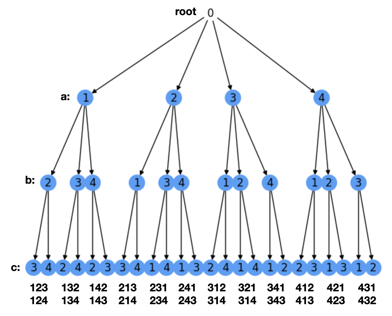
Fig. 2.2 Rooted tree where the leaves are the solutions to a counting problem.#
In particular, we have:
The root is the top parent node of the tree and it spans several children, thus forming the first level of siblings.
Each children is either a leaf (a node without children) or the parent of several children, thus forming the second level of siblings.
The process goes on until all the new siblings are leaves.
In our counting problem, we use a rooted tree to decompose the original counting task: how many one-to-one functions do we have between two sets of \(m\) and \(n\) elements, \(m\le n\)?
Each level in the tree (root not included) encodes a possible choice for each of the \(m\) variables. In the figure, \(m=3\) and we denote \(x_1\) by \(a\), \(x_2\) by \(b\) and \(x_3\) by \(c\). Therefore, in the first level we have \(n=4\) choices for \(a\): \(\{1,2,3,4\}\) (the children of the root).
In this problem does not matter neither the order of selection of the variables \(a\), \(b\), \(c\) nor that of the assignments. We simply follow a sistematic order: an increasing order both for variables (\(a,b,c\)) and assignments (\(1,2,3,4\)). However, the tree can be built/visited/traversed in three different ways. To better understand these ways, consider that a tree is a recursive structure, i.e. it is composed of subtrees. For instance, the root is composed of four subtrees \(T_1, T_2, T_3, T_4\) whose roots are the four possible asignments for variable \(a\). Then the traversals are:
Preorder. First visit the root. Then visit first (left) subtree \(T_1\) of the root in preorder before visiting the second subtree \(T_2\).
Inorder. First visit the first (left) sub-tree \(T_1\) of the root in inorder before visiting the root itself. After visiting the root, proceed to visit \(T_2\) in inorder, etc.
Postorder. First visit the first (left) subtree \(T_1\) of the root in postorder. Then, proceed to visit \(T_2\) in postorder, etc. Finally, visit the root.
However, there are two main traversals for solving in AI problems:
Depth-First-First (DFS). This is basically any of the above traversals. Following preorder, for instance, we build paths(sequences of nodes) such as \(\mathbf{123}\). Actually this is the first explored path in preorder. Then follow \(\mathbf{124}\), \(\mathbf{132}\), \(\mathbf{134}\ldots\) until \(\mathbf{431}\) and \(\mathbf{432}\). See the paths (not including the root) at the bottom of
perm.Breath-First-First (BFS). Given the root of the tree, visit the root of each of its subtrees (e.g. \(T_1, T_2, T_3, T_4\)). Then visit the roots of all the subtrees of \(T_1\) etc. All we do is to visit level \(l\) before visiting level \(l+1\). In BFS, all paths are expanded incrementally until we reach the leaves. For instance at level \(1\) (without counting the root) we have \(4\) incomplete paths: \(\mathbf{1}\ast\ast\), \(\mathbf{2}\ast\ast\), \(\mathbf{3}\ast\ast\) and \(\mathbf{4}\ast\ast\). Then we expand the subtrees from left to right and for the first subree we have: \(\mathbf{12}\ast\), \(\mathbf{13}\ast\) and \(\mathbf{14}\ast\ast\). Finally, at the leaves we have \(\mathbf{123}\), \(\mathbf{124}\), \(\mathbf{132}\), \(\mathbf{134}\ldots\) until \(\mathbf{431}\) and \(\mathbf{432}\).
2.2. Permutations and Combinations#
2.2.1. Linking Permutations and Combinations#
The aforementioned paths have no repeated nodes values, and thus are solutions to the counting problem. For instance the path \(\pi=\mathbf{124}\) means a function \(f_{\pi}\) where \(a=1,b=2,c=4\) and we left \(d\) unassigned. Therefore, the counting task is decomposed in \(m=3\) counting tasks (one per level): in the first level we can choose \(n\) values for \(a\); given that values, we can only choose \(n-1\) values for \(b\) and consequently \(n-2\) values for \(c\). As a result, the total number of one-to-one functions between \(X\) and \(Y\) is given by the the product rule \(n(n-1)(n-2)\) and this number is given by the \(P(n,r)\) r-permutation:
where in this case \(r=m\) (in general \(m\le n\)). Interestingly, for \(m=n\) (\(n\) levels in the tree) we have the classical permutation \(P(n,n)\) or simply \(P(n)\):
where \(!\) is the factorial and \(0!=1\). In combinatorics, permutations encode all the possible orders of \(n\) distinct elements. Actually, it is straightforward to prove that
In other words, r-permutations remove \((n-r)\) products (levels in the tree) from the full \(n!\) permutations. For instance, in the example in setfunction we only need to add \(1\) element (\(n-m =1\)) to \(X\) to make \(m=n\). This will result in \(1\) more level in the tree in rtree.
Combinations. What if in the above example, order does not matter? For instance, paths \(\mathbf{124}\),\(\mathbf{142}\), \(\mathbf{214}\), \(\mathbf{241}\), \(\mathbf{412}\) and \(\mathbf{421}\) are considered the same because they basically contain the same nodes \({1,2,4}\) in any possible order. This means that many groups of paths are in the tree of rtree.
An r-combination counts how many groups of \(r\) elements can be obtained from \(n\ge r\). It is defined as the number \(C(n,r)\):
Thus, looking at the definition of \(P(n,r)\) it becomes clear that \(C(n,r)\) remove \(r!(n-r)!\) from the numerator \(n!\). This is a good example of the so-called division rule: there are \(k/d\) ways of doing a task if it can be done in \(k\) ways and for each of these ways exacly \(d\) of the \(k\) ways are considered the same. In \(C(n,r)\), we have that \(k=n!/(n-r)!=P(n,r)\) and \(d=r!=P(r)\) since any of the \(P(n,r)\) paths in the tree can be done in \(r!\) ways if the order of the nodes does not matter. As a result:
2.2.2. Allowing repetitions#
In the our motivating example (finding injections \(f:X\rightarrow Y\)), each element of the \(Y\) set can be selected once in each different one-to-one function. Let us consider allowing repetition of any or some of the elements. This leads to more realistic counting problems (e.g. repeating letters to form codes, objects of the same variety, etc).
Suppose, for instance, that instead of enumerating the injective (one-to-one) functions between \(X\) and \(Y\), we ask how many functions \(f:X\rightarrow Y\) (one-to-one or not) do exist. The answer is simple once we realize that any element in \(X\) can be mapped (only once, given the definition of a function) to \(any\) of the elements of \(Y\). This consideration allows us to decompose the counting task as follows:
Consider first the element \(a\in X\) in
setfunction. It may be assigned to any element \(1,2,3,4\) of \(Y\). That is, for \(a\) we have \(n\) possible assignments.Similarly, for \(b\) and \(c\) we have the same number of assignments: \(n\).
As we have \(m\) elements in \(X\), the total number of assignments (functions) is \(n\cdot n\cdots n\) (\(m\) times), i.e. \(n^{m}\).
In terms of a tree-based representation, we will have an \(n-\)ary tree (\(n\) branches per level) with \(m\) levels (without counting the root). This tree has \(n^{m}\) leaves.
Therefore, a r-permutation with repetition is \(P_\sigma(n,r) = n^{r}\).
Sometimes, finding a \(P_\sigma(n,r)\) is not so straight and it needs a previous mapping or encoding scheme (this will be useful later to prove that a problem is NP-hard).
For instance, for finding all the possible subsets of a finite set \(S=\{1,2,\ldots,n\}\) (the size of the power set \({\cal P}^{S}\)), we start listing the elements:
Obviously \(\emptyset\) and \(S\) itself belong to \({\cal P}^{S}\). These sets are respectively the subset with \(O\) elements and that with all the \(n\) elements.
Next, we consider the subsets with \(1\) element: they are \(\{1\}, \{2\},\dots \{n\}\), i.e. \(n\).
Then, we consider the subsets with \(2\) elements. Since obviously order does not matter, i.e. \(\{i,j\}=\{j,i\}\), we have an r-combination: \({n\choose 2}\).
Similarly for counting the subsets with \(3,4,\dots, n-1\) elements we have \({n\choose 3}, {n\choose 4}\dots {n\choose n-1}\).
Since \(1={n\choose 0}={n\choose n}\) and \(n={n\choose 1}\), the size of the powerset is (we use the notation \(|.|\) to denote the size of something):
Herein we apply the sum rule: if there are \(n\) independent counting tasks, with \(s_i\) number of ways each, the total number of ways is \(\sum_{i=1}^ns_i\).
However, it is not so obvious that the sum of r-combinations is \(2^n\). We will clarify this point later on, when studying the Binomial theorem.
A much simpler (and clever) alternative, comes from encoding each subset as a binary string of \(n\) bits. For instance, \(\emptyset = 000\ldots 0\), whereas \(S = 111\ldots 1\). In between, we have that all the sets with \(2\) elements are encoded by the binary strings of length \(n\) with only \(2\) bits “on” (set to\(1\)s). Similarly for the sets of lengths \(3\ldots n-1\). As a result, there is a bijection between \({\cal P}^{S}\) and the binary numbers of \(n\) bits.
Obviously, the number of different strings with \(n\) bits is \(2^n\). In other words, we have two elements \(\{0,1\}\) which can be repeated insofar the number of total elements is \(n\). More formally, we have to find all the functions \(S:\rightarrow B\) between \(S=\{1,2,\ldots, n\}\) and the base set \(B=\{0,1\}\), i.e. \(P_\sigma(2,n) = 2^n\).
The above result can be generalized to any other base such as \(a\): \(a^n\). For instance the number of Navilens codes is \(4^n\), where \(n\) is the number of cells, since these codes have four colors: cyan, magenta, yellow and black (the white border facilitates only the automatic localization of the enclosing frame). Actually, \(4^n=(2\cdot 2)^n\gg 2^n\) and this is why Navilens codes are much denser than QR codes (even after discounting the checksum bits), i.e. we can represent much more codes with less bits.
2.2.3. Indistinguisable elements#
So far, the elements in the counting problem can be repeated. However, some counting problems rely on considering types of elements, instead of elements themselves. In other words, in some counting problems it does not matter the number of elements satisfying this or that property, it is more important to consider \(p\) elements of type \(a\), \(q\) elements of type \(b\) etc, and then accounting for the total number of ways. This is like impossing \(p\) zeros and \(q\) ones in in a string with \(n\) bytes, where \(p + q = n\).
Source problems. Consider the case where we have \(n\) sources (types), and we have \(r\le n\) ways of selecing them, where repeats are allowed. For instance, given \(n\) (elementwise unlimited) colors, we only have \(r\) ways of selecting them (maybe because our pallete of colors is blind to more than \(r\) colors).
2.2.3.1. Permutations with repetition#
If order matters, we have to clarify now many ways are allowable for each type. For instance, consider than there are \(n\) types of indistinguishable elements \(n_1 + n_2 +\ldots + n_p = n\).
Consider the following simple example. We are asked to find the ways of reordering the letters in the word “Tomorrow”. The length of the word is \(n=8\), but computing a permutation \(P(n)= n!\) is incorrect, since in permutations or r-permutations we assume that all the elements are different (to avoid over-counting). In other words, \(n!\) counts the word “Tomorrow” several times: \({n\choose 3}\) for the “o”s and \({n\choose 2}\) for the “r”s, since we have \(n_2=3\) “r”s and \(n_4=2\) “o”s (the rest of the letters “T”, “m” and “w”) appears only one: \(n_1 = n_3 = n_5 = 1\).
Summarizing, we have \(5\) types of letters in the word “Tomorrow” and \(n_1 + n_2 + n_3 + n_4 + n_5 = n\), i.e. \(1 + 3 + 1 + 2 + 1 = 8 = n\). Then, if we apply the product rule and decompose our problem in \(5\) counting tasks (as many as different types of letters), each of these tasks is a \(r-\)combination as follows:
We have \(n=8\) positions to fill.
Fill \(n_2=3\) positions with \({n \choose n_2=3}={8 \choose 3}\) combinations. We use combinations since once we select any of the groups of \(3\) positions, order does not matter inside the group.
Now we have \(n - n_2 = 8 - 3 = 5\) remaning positions to fill. Fill \(n_4=2\) of them with \({n - n_2\choose n_4}={5\choose 2}\) combinations.
Now there are \(n - n_2 - n_4 = 3\) positions left. As \(n_1 = n_3 = n_5 = 1\), take any order of them to make \({3\choose 1}\cdot {2\choose 1}\cdot {1\choose 1}\) combinations.
Finally, the product of all the above \(r-\)combinations leads to
Then, permutations with repetition \(P_{\sigma}(n)\) are defined as follows:
where we have \(p\) types of indistinguishable objects and \(n_1 + n_2 + \ldots n_p = n\).
The above definition can be also interpreted as follows. In the numerator we have all the permutations. However in the denominator we cancel some of them to avoid over-counting.
This is consistent with the definition of \(C(n,r)\) as \(P(n,r)/P(r)\). For instance, suppose that \(n_1\ge n_2\ge\ldots \ge n_p\).
2.2.3.2. Multisets#
Counting problems with repetitions, whatever there are indistinguishable elements or not, can be viewed from the angle of multisets. Why? Because a multiset is a generalization of a set where the elements are allowed to be repeated (we may even have infinite, i.e. \(\infty\), copies).
For instance, the letters in the word “Tomorrow” are encoded by the following multiset:
where \(n_1 = 1, n_2 = 3, n_3 = 1, n_4 = 2, n_5= 1\) and \(n_1 + n_2 + n_3 + n_4 + n_5 = n = 8\).
This allows us to better explain the number of permutations with repetitions (in the indistinguishable setting) as a product of combinations as we did in the previous section.
since we take first \(n_1\) positions with the first element of the multiset, then we take \(n_2\) of the remaining \(n - n_1\) positions with the second element of the multiset, etc.
In particular, when no repetitions are allowed all the elements in the (multi)set have just one copy: \(n_1 = n_2 =\ldots n_p = 1\). Then we have the definition of r-permutations:
Then, using now
\(P(n=5,r)\) gives the number of words of length \(r\le n\) that can be generated by using (once) the letters in \(S\). Of course, “Tomorrow” never appears!
In addition, we can use multisets to count r-permutations with repetition \(P_\sigma(n,r) = n^{r}\) in the distinguishable setting, simply by assuming that all the elements in the multiset have infinite copies, For instance let redefine \(S\) as
Then, we have \(n = 5\) elements with infinite copies each and \(r\) positions they can occupy, we now call these positions as boxes with infinity capacity:
Since we have infinite copies of “T”, “o”, “m”, “r” and “w”, we have
\(n\) choices to fill the first of the \(r\) positions.
Again, we have \(n\) choices to fill the second of the \(r\) positions, etc.
Then we have
In this latter case, “Tomorrow” appears if \(r=8\).
Summarizing so far, the permutations with repetition of a set are the permutations of a properly defined multiset!
2.2.3.3. Combinations with repetition#
Multisets are specially useful for defining combinations with repetition as combinations in a multiset.
First of all, remember than the meaning of the combinatorial number \({n\choose r}\) is the number of subsets of \(r-\)elements of any set of \(n\) (different) elements.
Consider, for instance the set \([n] = \{1,2,\ldots n\}\) (a very useful notation to use from now on). Then, \({n\choose 2}\) is the number of \(S_2\subseteq [n]\) with \(|S_2| = 2\), namely \(S_2=\{(1,2),(1,3),\ldots (1,n)\}\). In general, for \(S_r\subseteq [n]\), \(|S_r| = {n\choose r}\). Actually, we know that \(|S_0| + |S_1| + \ldots + |S_n| = 2^n\) due to the bijection between the power set and \(\{0,1\}^n\).
Therefore, in terms of binary coding, a set \(S_r\) is given by the bynary numbers of \(n\) bits with exactly \(r\) ones (and \(n-r\) zeros). Then, we can distribute the \(r\) among the \(n\) positions. Consequently, we will have \(n-r\) zeros distributed in blocks of \(x_i\) zeros each, that will be placed “before” and “after” every \(i\) position (denoted by \(1^i\)) of a \(1\):
Note that choosing the \(r\) positions for the ones among the \(n\) available slots determines the placement of the zeros. In other words, the positions of the ones indicates what elements of \([n]\) belongs to a given subset. This is simply the definition of the combinatorial number
where \(n_1 = r\), \(n_2 = (n-r)\) and \(n_1 + n_2 = n\). In other words, \({n\choose r}\) is the number of permutations of the multiset
Then, consider now the following multiset
where \(m = r + 1\). Then, the problem of finding all the sub-multisets of \(T\) of size say \(k = n - r\) can be posed in terms of finding the number of non-negative integer solutions to the equation
since we can solve this equation by taking \(x_i\ge 0\) of any of the \(m\) types, with the constraint that the sum of elements of all types is exactly \(k\). We quantify this as follows:
Therefore, in practice we only need \(x_i\le k\) (despite the number of copies in formally \(\infty\)). Indeed, finding a sub-multiset consist of mixing elements of some types \(x_i\) provided that the sum of all choices is \(k\).
In order to better visualize each sub-multiset, we consider \(x_i\) as a box of infinite capacity (in practice its maximum capacity is \(k\)). All the boxes are different and separated by a “\(+\)” which marks the change from box \(x_{i-1}\) to box \(x_{i}\) for \(i=2,\ldots,m\), i.e. we have \(m - 1\) separators.
This means that the \(m - 1\) separators must be taken into account although we cannot include them in the multiset \(T\) since they cannot be sequenced arbitrarily but appearing between two blocks/boxes \(x_{i-1}\) and \(x_{i}\).
To sum up, we have to count the number of \(k\)-combination of \(k + (m - 1)\) symbols (choosing exactly \(k\) elements). This number is defined as
and it is readed as “\(m\) multi-choose k”.
Interstingly, since \(m = r + 1\) and \(k = n - r\) we have
i.e. the number of \(n-\)bits numbers with exactly \(r\) bits set to one! (where \(n = m - 1\) and \(r = n - k\)).
The, the combinations with repetition \(C_{\sigma}(m,k)\) of \(k\) elements of \(m\) types are:
from the point of view of placing \(k\) elements of the multiset (with repetition), and
from the point of view of placing the \(m - 1\) markers (also with repetition but constrained to separate elements of different types).
Minimal Capacities. So far, the \(m\) elements of the multiset have infinite capacity but these capacities are not lower-bounded. However, what happens if all the elements of the multiset must satisfy \(x_i\ge a_i\)?
We want to find the non-negative integer solutions for the equation
Obviously, this problem also has a solution if \(a_i\le k\) for any \(a_i\). Then, the strategy to follow is to:
Give away \(a_i\) elements to \(x_i\) box.
Define new variables \(y_i = x_i - a_i\)
Let \(A = a_1 + a_2 + a_3 + \ldots a_m\). Then, the new problem to solve becomes finding the non-negative integer solutions of
Exercise. Find the number of ways of giving \(6\) oranges to \(3\) kids so that all kids has at least one orange.
We commence by identifying what are the boxes and what the elements. In this case, the \(3\) kids are the boxes and the \(6\) oranges are the elements to fill the boxes (one box per kid).
Then, the (basic) problem to solve is to find the non-negative integer solutions of \( x_1 + x_2 + x_3 = 6\;. \) The solution is \(C_{\sigma}(m=3,k=6) = \left(\!\!{m\choose k}\!\!\right) = {k + m - 1\choose k} = {6 + 3 - 1\choose 6} = {8\choose 6}= 8!/(6!\cdot 2!) = 28 \;.\)
However, this is not the solution to the problem. Since all kids must have at least one orange, we are interested in the solutions where \(x_i\ge 1\;\forall i\).
Then, we give \(1\) orange to each kid (we can do that because \(6\ge 3\)) and solve the following problem: \(y_1 + y_2 + y_3 = 6 - 1\cdot 3 = 3\), where \(y_i = x_i - 1\).
The solution is \(C_{\sigma}(m=3,k=3) = \left(\!\!{3\choose 3}\!\!\right) = {3 + 3 - 1\choose 3} = {3 + 3 - 1\choose 3} = {5\choose 3}= 5!/(3!\cdot 2!) = 10\;\). These solution (wrt the \(y_i\)s and mapped to \(x_i\) after undoing the change of variable) are:
\(
\begin{align}
& (1\;1\;1)\rightarrow (2\;2\;2)\\
& (2\;0\;1)\rightarrow (3\;1\;2)\\
& (2\;1\;0)\rightarrow (3\;2\;1)\\
& (1\;0\;2)\rightarrow (2\;1\;3)\\
& (1\;2\;0)\rightarrow (2\;3\;1)\\
& (0\;1\;2)\rightarrow (1\;2\;3)\\
& (0\;2\;1)\rightarrow (1\;3\;2)\\
& (3\;0\;0)\rightarrow (4\;1\;1)\\
& (0\;3\;0)\rightarrow (1\;4\;1)\\
& (0\;0\;3)\rightarrow (1\;1\;4)\\
\end{align}
\)
We can conclude that \(28 - 10 = 18\) solutions do not satisfy the requirement that each kid has at least one orange. These incorrect solutions are all where at least a kid has \(0\) oranges.
Note that the second part of the above exercise would have a different solution if no kid can have more than \(a\) oranges. This requires another strategy.
Maximal Capacities. If all boxes satify \(0\le x_i\le a_i\) (their capacity is upper bounded) we have multisets such as
i.e. we want to find the non-negative integer solutions for the equation
Count first the combinations with infinite capacities and then subtract the undeseriable combinations.
The undesirable combinations where \(x_i\) is involved satisfy \(x_i> a_i\), that is \(x_i\ge a_i + 1\).
Let us define \(A_i\) corresponding to \(x_i\) as:
We have \(A_1, A_2, \ldots, A_m\) multisets, each one corresponding to an inverse constraint \(x_i\ge a_i + 1\) and we want to count the number of combinations that DO NOT SATISFY ANY of the inverse constraints. In other words, this is equivalent to find the size of the set:
Computing \(|\bar{A}_1\cap \bar{A}_2\cap\ldots \cap\bar{A}_m|\) requires to use the inclusion-exclusion principle. Herein, we define it and later on we will explain it in detail. This principle simply comes from the generalizing the equation \(|A\cup B| = |A| + |B| - |A\cap B|\):
The above equation states that for counting the elements of a union of sets:
First count the elements of each set: \(|A_1| + |A_2| + \ldots\)
When doing so, if any pair of sets \(|A_i\cap A_j|>0\) this means that some element are over-counted when doing \(|A_j| + |A_j|\). Then, \(|A_i\cap A_j|\) should be discounted from the sum \(\sum_{i=1}^m|A_i|\).
Next, if any triplet of sets satisfies \(|A_i\cap A_j\cap A_k|>0\), where \(|A_i\cap A_j|>0\), this means that discounting that intersection must be compensated by adding \(|A_i\cap A_j\cap A_k|\).
Then, the progression continues by adding odd terms and subtracting even ones.
As a result, let \(S\) a given set (in our case, the set of all the combinations of the multiset with infinite capacity) and \(A_i\subseteq S\). Then, inclusion-exclusion principle is formulated as follows:
Them for counting these combinations we need to:
Compute all the \(|A_i|\) and sum them. In particular, we have
Compute all the \(|A_i\cap A_j|\) and discount them from the sum of \(|A_i|\)
And so on with \(|A_i\cap A_j\cap A_k|\), etc.
Lets do that in the following exercise.
Exercise. We have several types of balls: \(4\) of them are red (R), \(3\) are green (G) and \(2\) are blue (R). Find the number of ways of getting \(8\) balls.
We have the multiset \(T = \{4\cdot R, 3\cdot G, 2\cdot B\}\), i.e. \(m = 3\) (types of balls) and \(k = 8\) balls to take in total.
We have to find all the non-negative integer solutions of:
\(
x_1 + x_2 + x_3 = 8\;\text{s.t.}\; 0\le x_1\le 4, 0\le x_2\le 3,0\le x_3\le 2\;.
\)
Let us define the sub-multisets of the multiset with infinite capacity \(T^{\ast}=\{\infty\cdot R,\infty\cdot G, \infty\cdot B\}\) for the three constraints:
\(
\begin{align}
& A_1 = \text{Sub-multiset of size}\; 8\; \text{with}\; x_1\ge 5\;\\
& A_2 = \text{Sub-multiset of size}\; 8\; \text{with}\; x_2\ge 4\;\\
& A_3 = \text{Sub-multiset of size}\; 8\; \text{with}\; x_3\ge 3\;\;.
\end{align}
\)
Let \(S\) be the set of all the sub-multisets of size \(8\) of \(T^{\ast}\). Its size is the multi-choose
\(
|S| = \left(\!\!{m\choose k}\!\!\right) = \left(\!\!{3\choose 8}\!\!\right) = {10\choose 8} = 45\;.
\)
What is the size of each \(A_i\)? Well, by definition they are given by
\(
\begin{align}
|A_1| & = \left(\!\!{m\choose k - (a_1 + 1)}\!\!\right) = \left(\!\!{3\choose 8 - 5}\!\!\right) = \left(\!\!{3\choose 3}\!\!\right) = {5\choose 3}= 10\;.\\
|A_2| & = \left(\!\!{m\choose k - (a_2 + 1)}\!\!\right) = \left(\!\!{3\choose 8 - 4}\!\!\right) = \left(\!\!{3\choose 4}\!\!\right) = {6\choose 4}= 15\;.\\
|A_3| & = \left(\!\!{m\choose k - (a_3 + 1)}\!\!\right) = \left(\!\!{3\choose 8 - 3}\!\!\right) = \left(\!\!{3\choose 5}\!\!\right) = {7\choose 5}= 21\;.
\end{align}
\)
However, finding the sizes of the binary intersections \(|A_i\cap A_j|\) this may be not so straight. For \(A_1\cap A_2\) it is becase we must satisfy both \(x_1\ge 5\) and \(x_2\ge 4\) but this exceeds our budget which is \(k=8\) and then \(A_1\cap A_2 = \emptyset\). Then \(|A_1\cap A_2|=0\)
However, for \(A_1\cap A_3\) we have that the constraints are \(x_1\ge 5\) and \(x_3\ge 3\) and the sum of the upper bounds \(5 + 3 = 8\) is equal to the budget. Therefore, giving \(5 + 3\) balls to \(x_1\) and \(x_3\) forces \(x_2 = 0\) and we have a unique combination \((x_1=5, x_2 = 0, x_3=3)\). Therefore \(|A_1\cap A_3|=1\)
\(A_2\cap A_3\) must satisfy \(x_2\ge 4\) and \(x_3\ge 3\) and we have \(4 + 3 = 7\). After setting \(x_2 = 4\) and \(x_3 = 3\), we have solutions of the type \((r_1, 4 + r_2, 3 + r_3)\) that we can find by setting \(y_2 = 4 - x_2\), \(y_3 = 3 - x_3\) and finding the solutions of \(x_1 + y_2 + y_3 = 1\). The number of solutions is \(|A_2\cap A_3|=\left(\!\!{m\choose 1}\!\!\right) = \left(\!\!{3\choose 1}\!\!\right) = {3\choose 1}= 3\;.\)
Finally, \(A_1\cap A_2\cap A_3 = \emptyset\) and \(|A_1\cap A_2\cap A_3|= 0\;.\)
Summarizing, we have
\(
\begin{align}
|\bar{A_1}\cap\bar{A_2}\cap\bar{A_3}| &= |S| - (|A_1| + |A_2| + |A_3|) + (|A_1\cap A_2| + |A_1\cap A_3| + |A_2\cap A_3|) - A_1\cap A_2\cap A_3|\\
&= 45 - ( 10 + 15 + 21) + (0 + 1 + 3) - 0\\
&= 45 - 46 + 4 - 0 = 3\;.
\end{align}
\)
These solutions are: \((4,3,1)\), \((4,2,2)\) and \((3,3,2)\). Only these solutions satisfy
\(
x_1 + x_2 + x_3 = 8\;\text{s.t.}\; 0\le x_1\le 4, 0\le x_2\le 3,0\le x_3\le 2\;.
\)
i.e., the condition \(x_1 + x_2 + x_3 = 8\) forces us to report assignements close to the upper bounds.
2.3. The Principle of Exclusion-Inclusion#
The Exclusion-Inclusion Principle (PEI) is a powerful tool in counting problems with constraints, i.e. when we have to over-count (include) and then remove (exclude) counts. The PIE is very useful for our Discrete Brain (see the aforementioned problem of counting combinations with repetitions under constraints). It is often considered a “naive” way of solving counting problems with constraints because its complexity is \(O(2^n)\) but it is very useful to understand the combinatorial nature of a problem such as counting paths in a grid with forbidden positions as we will discover at the end of this section.
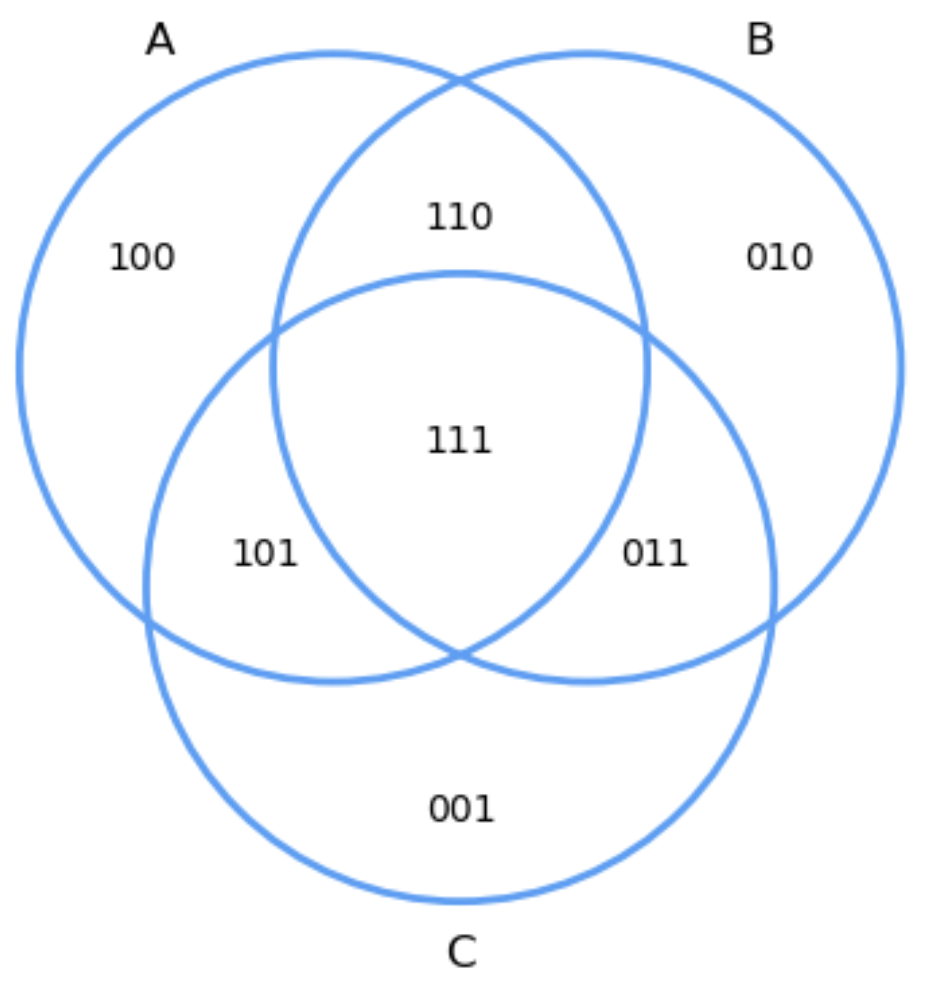
Fig. 2.3 Binary encoding of all subsets.#
Consider the general setting in PEI1, where we have \(m=3\) intersecting sets : \(A_1 = A\), \(A_2 = B\), \(A_3 = C\). We commence by choosing a
useful coding for each of the distinct subsets. For instance, \(100\) means the subset \(A_1\cap\bar{A}_2\cap\bar{A}_3\) (elements that only belong to \(A_1\)), where \(101\) means \(A_1\cap\bar{A}_2\cap A_3\).
Interestingly the aforementioned binary coding tells us how many times the elements in a given subset are over-counted (just take the numbers of ones in the code). This will be very useful from now on.
2.3.1. Discounting over-counts#
Now let us start by counting the elements of the union \(\bigcup_{i=1}^m A_i\) of \(m\) sets \(A_1,A_2,\ldots,A_m\) by simply summing the elements of the individual sets:
According to PEI1, the binary codes in each subset indicates how many times are counted the elements in that subset. This results in
\( A_1 = A = \{100, 110, 101, 111\}\;, A_2 = B = \{010, 011, 110, 111\}\;, A_3 = C = \{001, 101, 111, 011\} \)
i.e. so far our union can be see as the following multiset:
\( A_1\cup A_2\cup A_3 = \{100, 010, 001, 2\cdot 110, 2\cdot 101, 2\cdot 011, 3\cdot 111\} \)
Each \(A_i\) has elements counted once (\(1\) of them), twice (\(2\) of them) and three times (\(1\) of them).
One of the elements counted twice must be removed.
Two of the elements counted three times must be removed.
To remove the elements that are counted twice, we remove the elements in all pairwise intersections: \(A\cap B =\{110, 111\}\), \(A\cap C = \{101, 111\}\) and \(B\cap C = \{011, 111\}\) as indicated in PEIPairwise. Note that the subset \(111\) is removed three times.
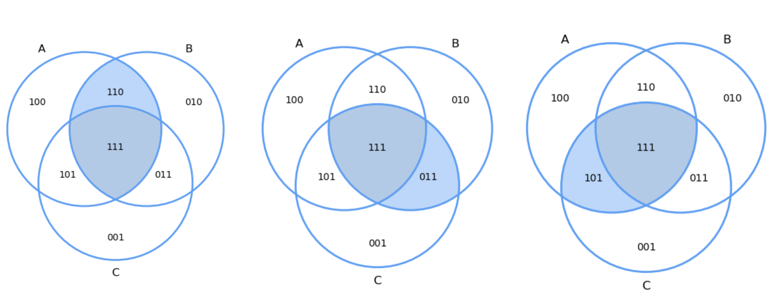
Fig. 2.4 Pairwise excluding intersections.#
More generally, we do
After removing the number of elements in the pairwise intersections, the resulting union is
\( A_1\cup A_2\cup A_3 = \{100, 010, 001, 110, 101,011\}\;. \) i.e. the three copies of \(111\) are removed. This is why a correct counting can be include back \(A_1\cap A_2\cap A_3 = \{111\}\).
More generally, for \(m=3\) we have:
For an arbitrary \(m\) we obtain:
We may formulate the above formula more compactly. To do that, note that the size of the intersection increases linearly (\(1,2,3,\ldots, m\))
We can be even more compact by realizing that the \(k-\)th term of the main sum relies on adding \({m\choose k}\) intersections.
This means that computing the size of the union is equivalent of computing all the possible subsets of \([m]=\{1,2,\ldots,m\}\) but the empty set and intersect them as follows:
Consequently, since we have to visit all the subsets of \([m]\), this naive way of computing the size of the union can be done in \(O(2^m)\).
2.3.2. Principle of Exclusion-Inclusion#
Once we have counted the size of the union of \(m\) sets, the PEI comes naturally: the number of elements which DO NOT BELONG to any of the sets \(A_1,A_2,\ldots, A_m\) (i.e. they belong to \(\bar{A}_1\cap \bar{A}_2\cap\ldots\cap \bar{A}_m\)) is given by:
where \(S\) is a set including all the \(A_i\) (the universal set). In our above example of PEI1, if \(S = \bigcup_{i=1}^m A_i\), then the intersection of complements \(\bar{A}_1\cap \bar{A}_2\cap\ldots\cap \bar{A}_m\) can be encoded by \(000\) and this means that it has no elements inside any Venn diagram!
2.3.3. Counting paths in grids#
One of the most interesting applications of the PEI in AI is path counting. Given a grid (later on we will define it more formally) we are interested in counting (and also in actually finding) the paths between two nodes of this grid, say \((0,0)\) and \((m,n)\).
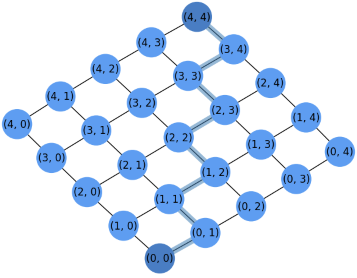
Fig. 2.5 Grid for counting paths between \((0,0)\) and \((4,4)\).#
In grid1 we show a grid where \(m=n=4\). A given node \((i,j)\) may be conected at most with \(4\) nodes: \((i+1,j)\) \((i,j+1)\), \((i-1,j)\) and \((i,j-1)\). This is why it is called a 4-grid because each node can have at most \(4\) neighbors.
However, for counting paths between the origin \((0,0)\) and the destination \((m=4,n=4)\) we are going to assume that these links are directed, i.e. a node \((i,j)\) can only travel either to \((i+1,j)\) or to \((i,j+1)\).
A path \(\Gamma\) is just a sequence (list) of nodes between the origin and the destination. For instance the path showed in grid1 is:
Interestingly, for drawing a path in the above grid we can only perform two types of movements from a given node \((i,j)\):
\(\Delta i\): \((i,j)\rightarrow (i+1,j)\).
\(\Delta j\): \((i,j)\rightarrow (i,j+1)\).
Then: How many paths do exist between \((0,0)\) and \((m,n)\)?
Since we have to arrive to \((m,n)\) from \((0,0)\) we need to make \(m\) movements of type \(\Delta i\) and \(n\) movements of type \(\Delta j\) in a given order!
Since order matters, we have to find permutations of \(m+n\) elements, where \(m\) of them are of type \(\Delta i\) and \(n\) of them are of type \(\Delta j\). We have permutations with repetition:
i.e., we can interpret the counting in terms of combinations, since we have \({m+n\choose m}\) ways of taking \(m\) elements of type \(\Delta i\) from \(m + n\) mixed elements, which is equivalent to the \({m+n\choose n}\) ways of taking \(n\) elements of type \(\Delta j\).
However, how is it applicable the PEI here?
Well, let use remove a node from the above grid, for instance the node \((2,2)\). As a result of removing \((2,2)\), the paper showed in grid1 cannot be built. Actually, the topology of the grid (the way its elements are connected independently of their layout, i.e. way we draw them) changes.
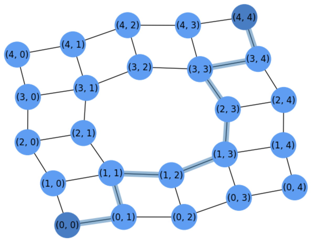
Fig. 2.6 Grid for counting paths between \((0,0)\) and \((4,4)\) after removing node \((2,2)\).#
For instance, when represeting the grid after removing the node \((2,2)\) we have to circumvent this node, through one of its neighbors as we show in grid2.
Then, the following question arises: How many paths do we have after removing a given node?
Well, let \(N_{ij}={i+j\choose i}\) be the number of paths that make \(i\) movements of type \(\Delta i\) and \(j\) movements of type \(\Delta j\).
Then, to find the number of paths in the grid of grid2, we should discount all the paths that visit the removed node \((2,2)\) from the universal set \(S_{\Gamma}\) of all paths between \((0,0)\) and \((4,4)\), whose size is \(N_{mn}=N_{44}={4 + 4\choose 4}=70\).
The number of paths that visit \((2,2)\) is given by the product of
The number of paths that go from \((0,0)\) to \((2,2)\): \(N_{22}\).
The number of paths that go from \((2,2)\) to \((2,2)\): \(N_{(4-2)(4-2)}=N_{22}\).
Then, we have
It is a good exercise to locate in grid1 the \(6\) paths going from \((0,0)\) to \((2,2)\) using \(2\) \(\Delta i\)-moves and \(2\) \(\Delta j\)-moves. One of these paths is
Therefore we have that the number of paths between \((0,0)\) and \((4,4)\) in in grid2 is
This is a naive application of the PEI, where \(|S| = N_{44}\).
However, let us remove a second node, say \((0,3)\). The new grid is in grid2:
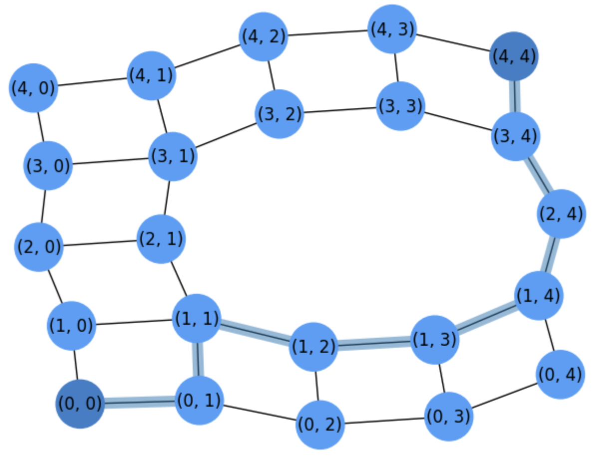
Fig. 2.7 Grid for counting paths between \((0,0)\) and \((4,4)\) after removing nodes \((2,2)\) and \((2,3)\).#
As we can see, the highlighted path passing through \((2,3)\) has been redirected and from \((1,3)\) we jump to \((1,4)\).
Then, What is the number of paths after removing both \((2,2)\) and \((2,3)\)?
Applying the PEI for \(m=2\) sets we have to consider:
\(A_1\): paths visiting node \((2,2)\).
\(A_2\): paths visiting node \((2,3)\).
Therefore, we are interested in the number:
We compute \(|A_2|\) as we computed \(|A_1|\).
The number of paths that visit \((2,3)\) is given by the product of
The number of paths that go from \((0,0)\) to \((2,3)\): \(N_{23}\)
The number of paths that go from \((2,3)\) to \((4,4)\): \(N_{(4-2)(3-2)}=N_{21}\).
Then, we have
Finally: How to count the paths in \(|A_1\cap A_2|\)?
The number of paths passing both through \((2,2)\) and \((2,3)\) can be calculated by the product of the paths going from \((0,0)\) to \((2,2)\), then going from \((2,2)\) to \((2,3)\) and (finally) reaching \((4,4)\) from there. These are:
Finally, we have:
Deleting nodes can be interpreted in terms of marking them as forbidden nodes (or obstacles when planning robot motion) as in grid1withobs
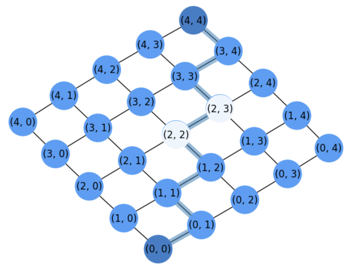
Fig. 2.8 Grid for counting paths between \((0,0)\) and \((4,4)\) after marking nodes \((2,2)\) and \((2,3)\) as forbidden or obstacles.#
In general, as we remove more and more nodes, \(m\) increases and computing the intersections may become more complex. Later on, we will describe simpler ways of actually counting these paths and extracting them.
Exercise. What happens in grid1withobs if we declare that node \((3,1)\) is also an obstacle?
We only have to discount the paths of \(A_3\) (passing through \((3,1)\)) since \(A_1\cap A_3 = A_2\cap A_3 = A_1\cap A_2\cap A_3 = \emptyset\).
We have:
\(
|A_3| = N_{31}\cdot N_{(4-3)(4-1)} = N_{31}\cdot N_{13} = {4 \choose 1}\cdot {4 \choose 3} = \frac{4!}{1!3!}\cdot \frac{4!}{3!1!} = 4\cdot 4 = 16\;.
\)
Therefore, we have
\(
\begin{align}
\# \Gamma &= N_{44} - (|A_1| + |A_2| + |A_3| - |A_1\cap A_2|)\\
&= N_{44} - (N_{22} + N_{23}\cdot N_{21} + N_{31}\cdot N_{13} - N_{22}\cdot N_{01}\cdot N_{21})\\
&= 70 - (36 + 30 + 16 - 18) = 70 - 64 = 6\;.
\end{align}
\)
It is a good additional exercise to identify why making \((3,1)\) an obstacle drops the count of paths from \(22\) to only \(6\). Basically, \((3,1)\) reduces to \(2\) the number of paths flowing through the right of the figure, since it is in the same row of \((2,2)\).
2.4. The Stirling’s formula#
Computing \(n!\) can be impossible to do in a computer as \(n\) increases. There are memory constrains because we need to store a product of \(n\) numbers and this may lead to stack overflow. There are also temporal constrains: even in the case of having infinite memory, computing two numbers of arbitrary length is not \(O(1)\). If \(n\) has length \(x\), it takes \(O(x^{\log_2 3})\) i.e. \(O(x^{1.58})\) using the Karatsuba divide-and-conquer algorithm (see Wikipedia article Karatsuba_algorithm). Interestingly, \(x=len(n)\) grows with \(O(\log_B n)\), where \(B\) is the base of \(x\). As a result, computing the factorial \(n!\) takes \(O(n\log n^{1.58})\).
Stirling’s proved that \(\text{as}\; n\rightarrow \infty, n!\approx \left(\frac{n}{e}\right)^n\sqrt{2\pi n}\;.\)
One may think that the above formula does not reduce the time complexity of the factorial since it involves a \(n^n\) product and obviouly \(n!<n^n\). However, for computing \(n^n\) (or in general \(a^n\), i.e. an power with a natural exponent) we exploit the fact that all the factors are equal (the base) and we may play with the exponents. Actually, we only need to perform \(O(\log_2 n)\), instead of \(n\), products to calculate \(n^n\).
Proof. An elegant way of proving the above assert is to estimate the minimal number of products needed to compute \(a^n\) for \(n\in\mathbb{N}\). This method is usually maned fast exponentiation or exponentiation by squaring. The intuition is as follows. When factorizing \(a^n\) in as few terms as possible: (1) if the term has an even power, \(a^{2k}\), take increasing values of \(k=2,4,8,\ldots\), and keep the same \(k\) as far as possible; (2) if eventually you need a term with an odd power take simply \(a\). For instance, for \(n=9\) make \(a^9 = a^4\cdot a^4\cdot a\).
The above rationale leads naturally to the following recurrence relation:
Consider the basic case where \(n=2^k\) is a power of \(2\), i.e. \(n_i\) is even at each call \(i\) to \(T\) but at the last one \(n_i=1\):
For instance, for \(n=128=2^7\) we have
Note that for \(n=2^k\) we make \(log_2(n) + 1=k + 1 \) calls. The \(k\) multiplications (discarding the last one) are the following
What happens if \(n\) is not a power of 2, say \(n=100\)?
we have \(k=7\) calls and \(\log_2(2^{k-1})\le \log_2(100)\le \log_2(2^{k})\). The products are
Note that we add an extra product when the recurrence reaches an odd \(n_i\) in the \(i-\)th call. In general we have \(O(\log_2 n)\) products. \(\square\)
Using the Stirling’s Formula. Back to the Stirling approximation of the factorial,
we have that both \(n^n\) (numerator) and \(e^n\) (denominator) can be computed efficiently. Similarly large combinatorial numbers such as \({2n\choose n}\) for large \(n\) can be computed efficiently as well (please try). In general the approximation of \(n!\) is very accurate even for small \(n\).
However the interest of the Stirling’s formula goes beyond efficiency considerations:
Simplicity. The formula is composed of simple functions and this may allow us to design/prove bounds for certain combinatorial numbers. Later on, we will show this in conjunction with Newton’s binomial theorem.
Complexity analysis. We now that \(O(n^n) > O(n!)\), but what does grow faster, \(e^n\) or \(n!\)?. The Stirling formula, or more precisely its logarithm, allows us to answer this question:
Herein, it is very useful to consider that for \(n\ge 2\) we have
and this leads to
Finally, since the log is a monotonic function of its argument, let us now consider the ratio of the logarithms
which is positive for \(n>1\). Therefore, \(O(n!) > O(e^n)\). \(\square\)
Information bounds. It is well known that the minimal number of comparions to sort \(n\) numbers using a comparison sort alorithm is \(\lceil \log(n!) \rceil\). The intuition is given by the mergesort algorithm: take recursively \(2\) sublists of \(n_i/2\) elements and when the lists have a single element return the merging of adjacent lists. The number of comparisons to merge two lists are no more than \(n_i\), and we have \(\log_2 n\) levels. Consequently, we perform at least \(n\log_2 n\) comparisons, i.e. we have \(\Omega(n\log_2 n)\approx \Omega(\log(n!))\).
Information theory, in particular the combinatorial definition of entropy.