
12. NetworkX#
NetworkX is a Python package for the creation, manipulation, and study of the structure, dynamics, and functions of complex networks. It provides data structures for networks, or graphs, as well as algorithms that can be used to analyze properties of those networks. The package is designed to allow the creation of networks and the analysis of their structure and function to be done in a few lines of code. It is used in a wide range of applications, from the analysis of social networks to the study of biological networks.
The rest of the course will be focused on the use of NetworkX to analyze and visualize networks. Also we will use the matplotlib package to visualize the networks. And finally, we will use the pandas package to manipulate the data and numpy to perform numerical operations. So, let’s start by installing the packages.
12.1. Installation#
To install the packages, you can use the following commands:
pip install networkx
To check if the installation was successful, you can run the following command:
pip show networkx
12.2. Importing the packages#
To import the packages, you can use the following commands:
import networkx as nx
12.3. Creating a graph#
To create a graph, you can use the following command:
G = nx.Graph() # This sentence creates an empty graph
print(G) # This gives as a output: Graph with 0 nodes and 0 edges
if you want to create a directed graph, you can use the following command:
G = nx.DiGraph() # This sentence creates an empty directed graph
print(G) # This gives as a output: DiGraph with 0 nodes and 0 edges
12.3.1. Creating a graph from numpy matrix#
To create a graph from a numpy matrix, you can use the following command:
import numpy as np
A = np.array([[0, 1, 0, 0, 0], [1, 0, 1, 0, 0], [0, 1, 0, 1, 0], [0, 0, 1, 0, 1], [0, 0, 0, 1, 0]]) # This creates a numpy matrix
G = nx.Graph(A) # This creates a graph from the numpy matrix
print(G.nodes) # This gives as a output: [0, 1, 2, 3, 4]
print(G.edges) # This gives as a output: [(0, 1), (1, 2), (2, 3), (3, 4)]
print(nx.adjacency_matrix(G).todense()) # This gives as a output: [[0 1 0 0 0]
                                         #                         [1 0 1 0 0]
                                         #                         [0 1 0 1 0]
                                         #                         [0 0 1 0 1]
                                         #                         [0 0 0 1 0]]
12.3.2. Creating a graph from pandas dataframe (easy way)#
To create a graph from a pandas dataframe, you can use the following command:
import pandas as pd
df = pd.DataFrame({'from': [0, 1, 2, 3, 4], 'to': [1, 2, 3, 4, 0]}) # This creates a pandas dataframe
G = nx.from_pandas_edgelist(df, 'from', 'to') # This creates a graph from the pandas dataframe
print(G.nodes) # This gives as a output: [0, 1, 2, 3, 4]
print(G.edges) # This gives as a output: [(0, 1), (1, 2), (2, 3), (3, 4), (0, 4)]
12.3.3. Adding nodes#
To add nodes to the graph, you can use the following command:
import networkx as nx
G = nx.Graph() # This sentence creates an empty directed graph
G.add_node(1) # This adds a node with the label 1
G.add_nodes_from([2, 3, 4, 5]) # This adds nodes with the labels 2, 3, 4, and 5
print(G.nodes) # This gives as a output: [1, 2, 3, 4, 5]
if you want to add nodes with attributes, you can use the following command:
color = {1: 'red', 2: 'blue', 3: 'green', 4: 'yellow', 5: 'black'} # We create a dictionary with the colors of the nodes
nx.set_node_attributes(G, color, 'color') # We set the colors of the nodes
print(G.nodes[1]) # This gives as a output: {'color': 'red'}
print(G.nodes[1]['color']) # This gives as a output: red
you can also create other types of attributes, such as weight, size, name, features, etc.
weight = {1: 1, 2: 2, 3: 3, 4: 4, 5: 5} # We create a dictionary with the weights of the nodes
nx.set_node_attributes(G, weight, 'weight') # We set the weights of the nodes
print(G.nodes[1]) # This gives as a output: {'color': 'red', 'weight': 1}
print(G.nodes[1]['weight']) # This gives as a output: 1
size = {1: 1, 2: 2, 3: 3, 4: 4, 5: 5} # We create a dictionary with the sizes of the nodes
nx.set_node_attributes(G, size, 'size') # We set the sizes of the nodes
print(G.nodes[1]) # This gives as a output: {'color': 'red', 'weight': 1, 'size': 1}
print(G.nodes[1]['size']) # This gives as a output: 1
name = {1: 'A', 2: 'B', 3: 'C', 4: 'D', 5: 'E'} # We create a dictionary with the names of the nodes
nx.set_node_attributes(G, name, 'name') # We set the names of the nodes
print(G.nodes[1]) # This gives as a output: {'color': 'red', 'weight': 1, 'size': 1, 'name': 'A'}
print(G.nodes[1]['name']) # This gives as a output: A
features = {1: [1, 2, 3], 2: [4, 5, 6], 3: [7, 8, 9], 4: [10, 11, 12], 5: [13, 14, 15]} # We create a dictionary with the features of the nodes
nx.set_node_attributes(G, features, 'features') # We set the features of the nodes
print(G.nodes[1]) # This gives as a output: {'color': 'red', 'weight': 1, 'size': 1, 'name': 'A', 'features': [1, 2, 3]}
print(G.nodes[1]['features']) # This gives as a output: [1, 2, 3]
12.3.4. Adding edges#
To add edges to the graph, you can use the following command:
G.add_edge(1, 2) # This adds an edge between the nodes 1 and 2
G.add_edges_from([(2, 3), (3, 4), (4, 5)]) # This adds edges between the nodes 2 and 3, 3 and 4, and 4 and 5
print(G.edges) # This gives as a output: [(1, 2), (2, 3), (3, 4), (4, 5)]
if you want to add edges with attributes, you can use the following command:
weight = {(1, 2): 1, (2, 3): 2, (3, 4): 3, (4, 5): 4} # We create a dictionary with the weights of the edges
nx.set_edge_attributes(G, weight, 'weight') # We set the weights of the edges
print(G.edges[1, 2]) # This gives as a output: {'weight': 1}
print(G.edges[1, 2]['weight']) # This gives as a output: 1
you can also create other types of attributes, such as color, size, name, features, etc.
color = {(1, 2): 'red', (2, 3): 'blue', (3, 4): 'green', (4, 5): 'yellow'} # We create a dictionary with the colors of the edges
nx.set_edge_attributes(G, color, 'color') # We set the colors of the edges
print(G.edges[1, 2]) # This gives as a output: {'weight': 1, 'color': 'red'}
print(G.edges[1, 2]['color']) # This gives as a output: red
size = {(1, 2): 1, (2, 3): 2, (3, 4): 3, (4, 5): 4} # We create a dictionary with the sizes of the edges
nx.set_edge_attributes(G, size, 'size') # We set the sizes of the edges
print(G.edges[1, 2]) # This gives as a output: {'weight': 1, 'color': 'red', 'size': 1}
print(G.edges[1, 2]['size']) # This gives as a output: 1
name = {(1, 2): 'A', (2, 3): 'B', (3, 4): 'C', (4, 5): 'D'} # We create a dictionary with the names of the edges
nx.set_edge_attributes(G, name, 'name') # We set the names of the edges
print(G.edges[1, 2]) # This gives as a output: {'weight': 1, 'color': 'red', 'size': 1, 'name': 'A'}
print(G.edges[1, 2]['name']) # This gives as a output: A
features = {(1, 2): [1, 2, 3], (2, 3): [4, 5, 6], (3, 4): [7, 8, 9], (4, 5): [10, 11, 12]} # We create a dictionary with the features of the edges
nx.set_edge_attributes(G, features, 'features') # We set the features of the edges
print(G.edges[1, 2]) # This gives as a output: {'weight': 1, 'color': 'red', 'size': 1, 'name': 'A', 'features': [1, 2, 3]}
print(G.edges[1, 2]['features']) # This gives as a output: [1, 2, 3]
12.3.5. Removing nodes and edges#
To remove nodes and edges from the graph, you can use the following commands:
G.remove_node(1) # This removes the node with the label 1
G.remove_nodes_from([2, 3, 4, 5]) # This removes the nodes with the labels 2, 3, 4, and 5
G.remove_edge(1, 2) # This removes the edge between the nodes 1 and 2
G.remove_edges_from([(2, 3), (3, 4), (4, 5)]) # This removes the edges between the nodes 2 and 3, 3 and 4, and 4 and 5
print(G.nodes) # This gives as a output: []
print(G.edges) # This gives as a output: []
12.3.6. Accessing nodes and edges#
To access the nodes and edges of the graph, you can use the following commands:
import networkx as nx
G = nx.Graph() # This sentence creates an empty directed graph
G.add_nodes_from([0,1, 2, 3, 4, 5]) # This adds nodes with the labels 1, 2, 3, 4, and 5
G.add_edges_from([(0, 2), (1, 2), (2, 3), (3, 4),(3,5)]) # This adds edges between the nodes 1 and 2, 2 and 3, 3 and 4, and 4 and 5
print(G.nodes) # This gives as a output: [0, 1, 2, 3, 4, 5]
print(G.edges) # This gives as a output: [(0, 2), (1, 2), (2, 3), (3, 4), (3, 5)]
print(list(G.nodes)[2]) # This gives as a output: 2
print(list(G.edges)[-1]) # This gives as a output: (3, 5)
12.3.7. Accessing the attributes of the nodes and edges#
To access the attributes of the nodes and edges of the graph, you can use the following commands:
import networkx as nx
G = nx.Graph() # This sentence creates an empty directed graph
G.add_nodes_from([0,1, 2, 3, 4, 5]) # This adds nodes with the labels 1, 2, 3, 4, and 5
G.add_edges_from([(0, 2), (1, 2), (2, 3), (3, 4),(3,5)]) # This adds edges between the nodes 1 and 2, 2 and 3, 3 and 4, and 4 and 5
color = {0: 'red', 1: 'blue', 2: 'green', 3: 'yellow', 4: 'black', 5: 'white'} # We create a dictionary with the colors of the nodes
nx.set_node_attributes(G, color, 'color') # We set the colors of the nodes
weight = {(0, 2): 1, (1, 2): 2, (2, 3): 3, (3, 4): 4, (3, 5): 5} # We create a dictionary with the weights of the edges
nx.set_edge_attributes(G, weight, 'weight') # We set the weights of the edges
print(G.nodes[0]) # This gives as a output: {'color': 'red'}
print(G.nodes[0]['color']) # This gives as a output: red
print(G.edges[0, 2]) # This gives as a output: {'weight': 1}
print(G.edges[0, 2]['weight']) # This gives as a output: 1
12.3.8. Accessing the neighbors of a node#
To access the neighbors of a node, you can use the following command:
import networkx as nx
G = nx.Graph() # This sentence creates an empty directed graph
G.add_nodes_from([0,1, 2, 3, 4, 5]) # This adds nodes with the labels 1, 2, 3, 4, and 5
G.add_edges_from([(0, 2), (1, 2), (2, 3), (3, 4),(3,5)]) # This adds edges between the nodes 1 and 2, 2 and 3, 3 and 4, and 4 and 5
print(list(G.neighbors(2))) # This gives as a output: [0, 1, 3]
12.3.9. Accessing the degree of a node#
To access the degree of a node, you can use the following command:
import networkx as nx
G = nx.Graph() # This sentence creates an empty directed graph
G.add_nodes_from([0,1, 2, 3, 4, 5]) # This adds nodes with the labels 1, 2, 3, 4, and 5
G.add_edges_from([(0, 2), (1, 2), (2, 3), (3, 4),(3,5)]) # This adds edges between the nodes 1 and 2, 2 and 3, 3 and 4, and 4 and 5
print(G.degree(2)) # This gives as a output: 3
12.3.10. Accessing the number of nodes and edges#
To access the number of nodes and edges of the graph, you can use the following commands:
import networkx as nx
G = nx.Graph() # This sentence creates an empty directed graph
G.add_nodes_from([0,1, 2, 3, 4, 5]) # This adds nodes with the labels 1, 2, 3, 4, and 5
G.add_edges_from([(0, 2), (1, 2), (2, 3), (3, 4),(3,5)]) # This adds edges between the nodes 1 and 2, 2 and 3, 3 and 4, and 4 and 5
print(G.number_of_nodes()) # This gives as a output: 6
print(G.number_of_edges()) # This gives as a output: 5
12.3.11. Accessing the adjacency matrix#
To access the adjacency matrix of the graph, you can use the following command:
import networkx as nx
G = nx.Graph() # This sentence creates an empty directed graph
G.add_nodes_from([0,1, 2, 3, 4, 5]) # This adds nodes with the labels 1, 2, 3, 4, and 5
G.add_edges_from([(0, 2), (1, 2), (2, 3), (3, 4),(3,5)]) # This adds edges between the nodes 1 and 2, 2 and 3, 3 and 4, and 4 and 5
print(nx.adjacency_matrix(G).todense()) # This gives as a output: [[0 0 1 0 0 0]
                                            #                         [0 0 1 0 0 0]
                                            #                         [1 1 0 1 0 0]
                                            #                         [0 0 1 0 1 1]
                                            #                         [0 0 0 1 0 0]
                                            #                         [0 0 0 1 0 0]]
12.3.12. Accessing the degree matrix#
To access the degree matrix of the graph, you can use the following command:
import networkx as nx
import numpy as np
g = nx.Graph()
g.add_nodes_from([1,2,3,4,5,6])
g.add_edges_from([(1,2),(4,5),(2,6),(2,4),(1,3),(3,5)])

# Obtener los grados de cada nodo
degrees = dict(g.degree())

n = len(g.nodes())
degree_matrix = np.zeros((n, n))

# Rellenar la diagonal con los grados de cada nodo
for i, node in enumerate(sorted(g.nodes())): # El enumerate que vimos en clase.
    degree_matrix[i, i] = degrees[node]

print(degree_matrix) # This gives as a output: [[1 0 0 0 0 0]
                                      #                         [0 1 0 0 0 0]
                                      #                         [0 0 3 0 0 0]
                                      #                         [0 0 0 3 0 0]
                                      #                         [0 0 0 0 1 0]
                                      #                         [0 0 0 0 0 1]]
12.3.13. Accessing the Laplacian matrix#
To access the Laplacian matrix of the graph, you can use the following command:
import networkx as nx
G = nx.Graph() # This sentence creates an empty directed graph
G.add_nodes_from([0,1, 2, 3, 4, 5]) # This adds nodes with the labels 1, 2, 3, 4, and 5
G.add_edges_from([(0, 2), (1, 2), (2, 3), (3, 4),(3,5)]) # This adds edges between the nodes 1 and 2, 2 and 3, 3 and 4, and 4 and 5
print(nx.laplacian_matrix(G).todense()) # This gives as a output: [[ 1  0 -1  0  0  0]
                                                                    # [ 0  1 -1  0  0  0]
                                                                    # [-1 -1  3 -1  0  0]
                                                                    # [ 0  0 -1  3 -1 -1]
                                                                    # [ 0  0  0 -1  1  0]
                                                                    # [ 0  0  0 -1  0  1]]
12.4. Visualizing the graph#
To visualize the graph, we are going to use matplotlib and the command nx.draw. This command takes 2 important parameters: the graph and the position of the nodes. The position of the nodes is a dictionary where the keys are the nodes and the values are the positions of the nodes. The positions of the nodes can be calculated using the commands nx.spring_layout, nx.kamada_kawai_layout,etc. You can check more details in the official documentation.
import matplotlib.pyplot as plt
plt.figure(figsize=(8, 5)) # This sets the size of the figure
G = nx.Graph() # This creates an empty graph
G.add_nodes_from([0,1, 2, 3, 4, 5]) # This adds nodes with the labels 1, 2, 3, 4, and 5
G.add_edges_from([(0, 2), (1, 2), (2, 3), (3, 4),(3,5)]) # This adds edges between the nodes 1 and 2, 2 and 3, 3 and 4, and 4 and 5
pos = nx.spring_layout(G, seed=42) # This calculates the positions of the nodes with a seed
nx.draw(G, pos) # This draws the graph with the calculated positions
plt.show() # This shows the graph
The output of the previous code is the following graph:
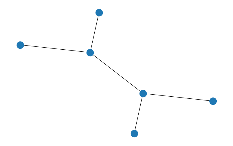
Fig. 12.1 Output of the plot#
This is the most basic way to visualize a graph. We can make more complex visualizations using the parameters of the nx.draw command. For example, we can change the color of the nodes and the edges, the size of the nodes, the width of the edges, the opacity of the nodes and the edges, the shape of the nodes, the border of the nodes, etc. You can check more details in the official documentation.
Here is an example of a more complex visualization:
import matplotlib.pyplot as plt
plt.figure(figsize=(8, 5)) # This sets the size of the figure
plt.title('Graph', fontsize=15, color='black', fontweight='bold', style='italic') # This sets the title of the graph
G = nx.Graph() # This creates an empty graph
G.add_nodes_from([0,1, 2, 3, 4, 5]) # This adds nodes with the labels 1, 2, 3, 4, and 5
G.add_edges_from([(0, 2), (1, 2), (2, 3), (3, 4),(3,5)]) # This adds edges between the nodes 1 and 2, 2 and 3, 3 and 4, and 4 and 5
pos = nx.spring_layout(G, seed=42) # This calculates the positions of the nodes with a seed
nx.draw(G, pos, node_color='red',
        node_size=500, node_shape='o',
        alpha=0.8, edge_color='black',
        width=2, style='dashed', font_size=12,
        font_color='black', font_weight='bold',
        font_family='serif', with_labels=True) # This draws the graph with the calculated positions
plt.show() # This shows the graph
The output of the previous code is the following graph:
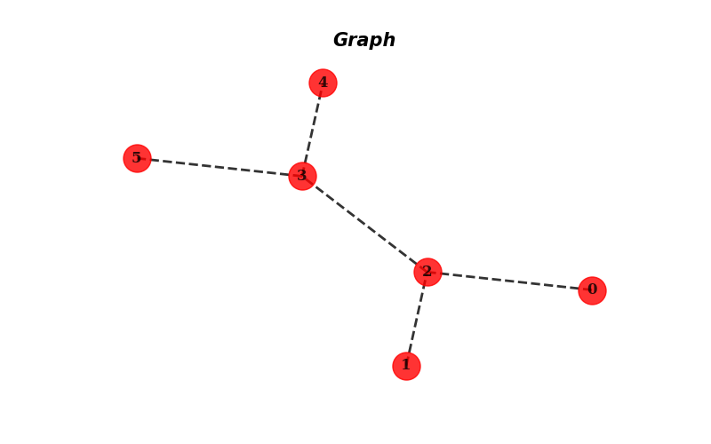
Fig. 12.2 Output of the plot#
Let’s step a little bit further and create a more complex graph. We are going to create a graph with 10 nodes and 15 edges. Also each node will have a color based on the class of the node, different sizes based on the degree of the node. Edges will be different styled based on if they connect nodes with the same class or different classes.
import matplotlib.pyplot as plt
import networkx as nx
plt.figure(figsize=(8, 5)) # This sets the size of the figure
plt.title('Graph', fontsize=15, color='black', fontweight='bold') # This sets the title of the graph
G = nx.Graph() # This creates an empty graph
G.add_nodes_from([0,1, 2, 3, 4, 5, 6, 7, 8, 9]) # This adds nodes with the labels 1, 2, 3, 4, and 5
G.add_edges_from([(0, 2), (1, 2), (2, 3), (3, 4),(3,5), (0, 6), (1, 7), (2, 8), (3, 9), (4, 5), (6, 7), (7, 8), (8, 9), (9, 6), (6, 5)]) # This adds edges between the nodes 1 and 2, 2 and 3, 3 and 4, and 4 and 5
labels_dict = {0: 'A', 1: 'A', 2: 'A', 3: 'C', 4: 'C', 5: 'B', 6: 'B', 7: 'B', 8: 'D', 9: 'D'} # We create a dictionary with the labels of the nodes
nx.set_node_attributes(G, labels_dict, 'label') # We set the labels of the nodes
edge_labels = {(0, 2): 'friend', (1, 2): 'friend', (2, 3): 'family', (3, 4): 'family', (3, 5): 'family', (0, 6): 'friend', (1, 7): 'friend', (2, 8): 'family', (3, 9): 'family', (4, 5): 'friend', (6, 7): 'friend', (7, 8): 'family', (8, 9): 'family', (9, 6): 'friend', (6, 5): 'friend'}
nx.set_edge_attributes(G, edge_labels, 'relation') # We set the labels of the edges
pos = nx.spring_layout(G, seed=42) # This calculates the positions of the nodes with a seed
# This is the non-fancy way to create the colors
colors = []
for node in G.nodes():
    if G.nodes[node]['label'] == 'A':
        colors.append('red')
    elif G.nodes[node]['label'] == 'B':
        colors.append('blue')
    elif G.nodes[node]['label'] == 'C':
        colors.append('yellow')
    else:
        colors.append('black')
# This is the fancy way to create the colors, by using mapcolors that offers matplotlib
# We map each label of the nodes to a color
colors = []
for node in G.nodes():
    if G.nodes[node]['label'] == 'A':
        colors.append(0)
    elif G.nodes[node]['label'] == 'B':
        colors.append(1)
    elif G.nodes[node]['label'] == 'C':
        colors.append(2)
    else:
        colors.append(3)
# We create the sizes of the nodes
sizes = []
for node in G.nodes():
     # Based on the degree of the node, we assign a size
     sizes.append(G.degree[node]*300)
# We create the styles of the edges
edge_styles = []
for edge in G.edges():
    if G.edges[edge]['relation'] == 'friend':
        edge_styles.append('dashed')
    else:
        edge_styles.append('solid')
nx.draw_networkx_nodes(G, pos, node_color=colors,
                    cmap=plt.cm.tab10, node_size=sizes,
                    alpha=0.8) # This draws the nodes with the calculated positions
nx.draw_networkx_edges(G, pos, edge_color='black', width=2, style=edge_styles)
nx.draw_networkx_labels(G, pos, font_size=12,
                        font_color='black', font_weight='bold',
                        font_family='serif') # This draws the labels with the calculated positions
nx.draw_networkx_edge_labels(G, pos, edge_labels=edge_labels, font_size=12,
                            font_color='black', font_weight='bold',
                            font_family='serif') # This draws the edge labels with the calculated positions
plt.axis('off') # This turns off the axis
plt.show() # This shows the graph
The output of the previous code is the following graph:
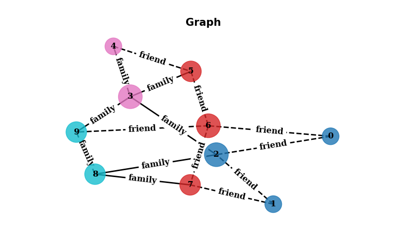
Fig. 12.3 Output of the plot#
12.5. Conclusion#
In this section, we have learned how to create a graph, add nodes and edges, access the nodes and edges, access the attributes of the nodes and edges, access the neighbors of a node, access the degree of a node, access the number of nodes and edges, access the adjacency matrix, access the degree matrix, access the Laplacian matrix, and visualize the graph. In the next section, we will learn how to analyze the graph and perform some operations on the graph.
12.6. Exercises#
12.6.1. Exercise 1#
After reading the previous section, you should be able to create your first Jupyter-Notebook and write a report about all the things you have learned in this section. In order to have a good structure, we recommend you to follow exactly the same structure as in this notebook.
12.6.2. Exercise 2#
After what we saw in class, you should be able to your own graph from your pandas dataframe. Once you have created the graph, you should be able to visualize it in the best way possible.
Hint
This is temporally
# Now we are going to performe a random walk on the graph
import matplotlib.pyplot as plt
import pandas as pd
import numpy as np
import networkx as nx

print("Creating the graph")
# Create a NumPy array
data = np.array([
    [1,'Alice', 25, 'New York', [3]],
    [2,'Bob', 30, 'Los Angeles' ,[3]],
    [3,'Charlie', 35, 'Chicago', [1,2,4]],
    [4,'David', 40, 'Houston', [3,5,6]],
    [5,'Emily', 45, 'Phoenix', [4]],
    [6,'Frank', 50, 'Philadelphia', [4]]
],dtype=object)

# Create a DataFrame from the NumPy array
df = pd.DataFrame(data, columns=['id','name','age','city','friends'])
12.7. Submission#
For the delivery of the practice 2, what you will be asked to do is to make a zip (name_name.zip) containing 3 notebooks: a first notebook containing the pandas section, a second notebook containing how you have done the visualizations and a third notebook representing the networkx part. Also it is important to add to the zip the pandas dataset you have created and the 4 figures
At the end the zip should be like this when you unzip it:
name_surname.zip
├── pandas.ipynb
├── matplotlib.ipynb
└── networkx.ipynb
└── dataset.csv
└── visualization1.png
└── visualization2.png
└── visualization3.png
└── visualization4.png