
21. Assignment 07/24#
21.1. Counting groups#
Exercise a) How many groups of up to \(3\) different elements can we form with \(10\) individuals (including a group with no-one)?
b) How many groups of more than \(3\) different elements can we form with \(10\) individuals?
a) For this simple exercise it is essential to understand that “forming a group of \(k\) different elements from \(n\) elements” is simply \({n\choose k}=\frac{n!}{k!(n-k)!}\).
However, we are asked to count how many groups of \(k=0,1,2,3\) elements do we have. Since each group is different from the others, we have that this number, for \(n=10\), is
\(
N_k={n\choose 0} + {n\choose 1} + {n\choose 2} + {n\choose 3} = {10\choose 0} + {10\choose 1} + {10\choose 2} + {10\choose 3} = 1 + 10 + 45 + 120 = 176\;.
\)
b) For \(k>3\) elements, we have to count \({n\choose 4}+{n\choose 5}+\ldots+{n\choose 10}\) but this solution requires a lot of calculus. In theory, we studied that \({n\choose k}\) counts the number of subsets of size \(k\) in a set of \(n\) elements. This means that \({n\choose 0}+{n\choose 1}+\ldots+{n\choose n}=2^n\).
Then, the number of groups with more than \(k=3\) elements is simply
\(
N_{k>}=2^n - N_k = 2^{10} - 176 = 1024 - 176 = 848\;.
\)
21.2. Bernouilli trials#
Exercise
Consider the following Bernouilli trial: Throw \(2\) dices simultaneously and register the outcomes as \((x,y)\). Then infer \(p\) and \(q\), where \(p + q = 1\) in the following case:
\(
\begin{align}
\;\;\text{a)}\;\; p &= \{\text{Prob. of}\;\; |x-y|>0 \;\;\text{is even}\}\\
\;\;\text{b)}\;\; p &= \{\text{Prob. of}\;\; \frac{x}{y} \;\;\text{is integer}\}\\
\end{align}
\)
and give also the expectations and variances of the Bernouilli variables associated with these experiments.
Firstly, the sample space \(\Omega\) is given by the cartesian product \(\Omega = \{1,\ldots,6\}\times \{1,\ldots,6\}\). Thus, we have
\(
\Omega = \begin{matrix}
(1,1) & (1,2) & (1,3) & (1,4) & (1,5) & (1,6) \\
(2,1) & (2,2) & (2,3) & (2,4) & (2,5) & (2,6) \\
(3,1) & (3,2) & (3,3) & (3,4) & (3,5) & (3,6) \\
(4,1) & (4,2) & (4,3) & (4,4) & (4,5) & (4,6) \\
(5,1) & (5,2) & (5,3) & (5,4) & (5,5) & (5,6) \\
(6,1) & (6,2) & (6,3) & (6,4) & (6,5) & (6,6) \\
\end{matrix}
\)
Thus, we have the sample spaces for the random variables \(X=\{|x-y|:(x,y)\}\) and \(Y=\{x/y:(x,y)\}\):
\(
\Omega_{X} = \begin{matrix}
0 & 1 & 2 & 3 & 4 & 5\\
1 & 0 & 1 & 2 & 3 & 4\\
2 & 1 & 0 & 1 & 2 & 3\\
3 & 2 & 1 & 0 & 1 & 2\\
4 & 3 & 2 & 1 & 0 & 1\\
5 & 4 & 3 & 2 & 1 & 0\\
\end{matrix}
\)
\(
\Omega_{Y} = \begin{matrix}
1 & \frac{1}{2} & \frac{1}{3} & \frac{1}{4} & \frac{1}{5} & \frac{1}{6}\\
2 & 1 & \frac{2}{3} & \frac{2}{4} & \frac{2}{5} & \frac{2}{6}\\
3 & \frac{3}{2} & 1 & \frac{3}{4} & \frac{3}{5} & \frac{3}{6}\\
4 & 2 & \frac{4}{3} & 1 & \frac{4}{5} & \frac{4}{6}\\
5 & \frac{5}{2} & \frac{5}{3} & \frac{5}{4} & 1 & \frac{5}{6}\\
6 & 3 & 2 & \frac{6}{4} & \frac{6}{5} & 1\\
\end{matrix}
\)
a) For \(\Omega_{X}\) we have a symmetric matrix with zeros in the diagonal. Therefore we have \(6\) cases not included in the definition \(|x-y|>0\): the ones in the diagonal, where \(x=y\). Then, we proceed to count the odd entries per row:
\(
\begin{align}
\text{Row 1}&=3\;\;\text{odd entries}\\
\text{Row 2}&=3\;\;\text{odd entries}\\
\text{Row 3}&=3\;\;\text{odd entries}\\
\text{Row 4}&=3\;\;\text{odd entries}\\
\text{Row 5}&=3\;\;\text{odd entries}\\
\text{Row 6}&=3\;\;\text{odd entries}\\
\end{align}
\)
This is not surprising since in each row we have a \(0\) entry, \(3\) odd entries and only \(2\) even entries. This results in \(p = \frac{2\cdot 6}{36}=\frac{12}{36}=\frac{1}{3}\), i.e. only one-third of the dice throws satisfy the condition “\(|x-y|>0\; \text{is odd}\)”.
As a result
\(
\begin{align}
&\;E(X_{even}) = 1\cdot p + 0\cdot q = p = \frac{1}{3}\;.\\
& Var(X_{even}) = E(X_{even}^2) - E(X_{even})^2 = p - p^2 = p(1-p) = pq = \frac{1}{3}\cdot\frac{2}{3} = \frac{2}{9}\:.
\end{align}
\)
b) For \(\Omega_{Y}\) we have an asymmetric matrix with ones in the diagonal. Therefore we have at least \(6\) cases included in the definition “\(\frac{x}{y}\;\text{is integer}\)”: the ones in the diagonal, where \(x=y\).
In addition, the first column has all its entries integer. Then, we add \(6\) more favorable cases.
For the rest of the matrix, we have only \(3\) more cases of integer divisions: \(\frac{4}{2}=2,\frac{6}{2}=3\) and \(\frac{6}{3}=2\).
As a result, \(p=\frac{6+5+3}{36}=\frac{14}{36}=\frac{7}{18}=0.39\).
\(
\begin{align}
&\;E(Y_{integer}) = 1\cdot p + 0\cdot q = p = \frac{7}{18}=0.39\;.\\
& Var(Y_{integer}) = E(Y_{integer}^2) - E(Y_{integer})^2 = p - p^2 = p(1-p) = pq = 0.39\cdot 0.61 = 0.2379\:.
\end{align}
\)
21.3. Random Walks on Graphs#
Exercise. Given the escape room in the In Fig. 21.1 we plot a triangular mesh where the outputs (border nodes or absorbing states) are marked as \(1\) and \(0\) indicating respectively “success” and “failure”. What are the probabilities that random walks launched from the interior nodes \(x_1\), \(x_2\), and \(x_3\), succeed?. Set the system and perform \(3\) iterations starting from \(\mathbf{x}^0=[1\;1\;1]^T\). Explain the results.
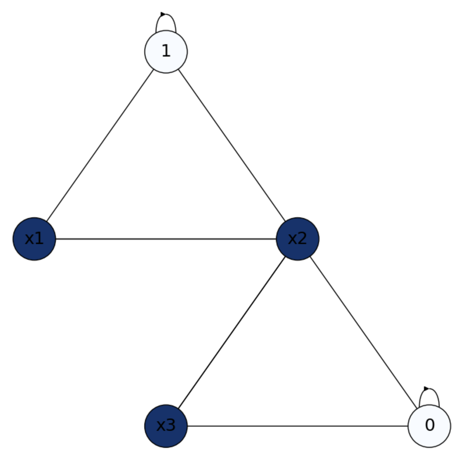
Fig. 21.1 Triangular mesh with interior nodes \(x_1\),\(x_2\) and \(x_3\).#
Let us formulate the matrices \(\mathbf{Q}\) (probabilities between interior nodes) and \(\mathbf{R}\) (probabilities between interior and absorbing nodes). From \(n_B = 2\) and \(n_I = 3\), we have
\(
\mathbf{Q}_{3} =
\begin{bmatrix}
0 & \frac{1}{2} & 0 \\
\frac{1}{4} & 0 & \frac{1}{4} \\
0 & \frac{1}{2} & 0 \\
\end{bmatrix}
\)
\(
\mathbf{R}_{3\times 2} =
\begin{bmatrix}
\frac{1}{2} & 0 \\
\frac{1}{4} & \frac{1}{4} \\
0 & \frac{1}{2}\\
\end{bmatrix}
\)
Then, from \(f_B = [1\;0]^T\) and \(f_D = [x_1\;x_2\;x_3]^T\) we set the system
\(
\underbrace{(\mathbf{I}_{3}-\mathbf{Q})}_{\mathbf{A}}\underbrace{f_D}_{\mathbf{x}} = \underbrace{\mathbf{R}f_B}_{\mathbf{b}}\;
\)
as follows
\(
\begin{bmatrix}
1 & -\frac{1}{2} & 0\\
-\frac{1}{4} & 1 & -\frac{1}{4} \\
0 & -\frac{1}{2} & 1\\
\end{bmatrix}
\begin{bmatrix}
x_1\\
x_2\\
x_3\\
\end{bmatrix} =
\begin{bmatrix}
\frac{1}{2} & 0 \\
\frac{1}{4} & \frac{1}{4} \\
0 & \frac{1}{2}\\
\end{bmatrix}
\begin{bmatrix}
1\\
0\\
\end{bmatrix}
\)
i.e.
\(
\begin{bmatrix}
1 & -\frac{1}{2} & 0\\
-\frac{1}{4} & 1 & -\frac{1}{4} \\
0 & -\frac{1}{2} & 1\\
\end{bmatrix}
\begin{bmatrix}
x_1\\
x_2\\
x_3\\
\end{bmatrix} =
\begin{bmatrix}
\frac{1}{2}\\
\frac{1}{4}\\
0 \\
\end{bmatrix}
\)
Let us now set and solve the iterative system via Jacobi for this problem:
\(
\mathbf{x}^{t+1} = \mathbf{b} - (\mathbf{L} + \mathbf{U})\mathbf{x}^{t}\;.
\)
\(
\begin{bmatrix}
\mathbf{x}_1^{t+1}\\
\mathbf{x}_2^{t+1}\\
\mathbf{x}_3^{t+1}\\
\end{bmatrix} =
\begin{bmatrix}
\frac{1}{2}\\
\frac{1}{4}\\
0\\
\end{bmatrix}-
\begin{bmatrix}
0 & -\frac{1}{2} & 0 \\
-\frac{1}{4} & 0 & -\frac{1}{4}\\
0 & -\frac{1}{2} & 0\\
\end{bmatrix}
\begin{bmatrix}
\mathbf{x}_1^{t}\\
\mathbf{x}_2^{t}\\
\mathbf{x}_3^{t}\\
\end{bmatrix}
\)
Thus, setting \(\mathbf{x}_0 = [1\;1\;1]^T\) we have the first iteration:
\(
\begin{bmatrix}
\mathbf{x}_1^{1}\\
\mathbf{x}_2^{1}\\
\mathbf{x}_3^{1}\\
\end{bmatrix} =
\begin{bmatrix}
\frac{1}{2}\\
\frac{1}{4}\\
0\\
\end{bmatrix}-
\begin{bmatrix}
0 & -\frac{1}{2} & 0 \\
-\frac{1}{4} & 0 & -\frac{1}{4}\\
0 & -\frac{1}{2} & 0\\
\end{bmatrix}
\begin{bmatrix}
1\\
1\\
1\\
\end{bmatrix} =
\begin{bmatrix}
\frac{1}{2}\\
\frac{1}{4}\\
0\\
\end{bmatrix}-
\begin{bmatrix}
-\frac{1}{2}\\
-\frac{2}{4}\\
-\frac{1}{2}\\
\end{bmatrix} =
\begin{bmatrix}
1\\
\frac{3}{4}\\
\frac{1}{2}\\
\end{bmatrix}\;.
\)
Then the second:
\(
\begin{bmatrix}
\mathbf{x}_1^{2}\\
\mathbf{x}_2^{2}\\
\mathbf{x}_3^{2}\\
\end{bmatrix} =
\begin{bmatrix}
\frac{1}{2}\\
\frac{1}{4}\\
0\\
\end{bmatrix}-
\begin{bmatrix}
0 & -\frac{1}{2} & 0 \\
-\frac{1}{4} & 0 & -\frac{1}{4}\\
0 & -\frac{1}{2} & 0\\
\end{bmatrix}
\begin{bmatrix}
1\\
\frac{3}{4}\\
\frac{1}{2}\\
\end{bmatrix} =
\begin{bmatrix}
\frac{1}{2}\\
\frac{1}{4}\\
0\\
\end{bmatrix}-
\begin{bmatrix}
-\frac{3}{8}\\
-\frac{3}{8} \\
-\frac{3}{8}\\
\end{bmatrix} =
\begin{bmatrix}
\frac{7}{8}=0.875\\
\frac{5}{8}=0.625\\
\frac{3}{8}=0.375\\
\end{bmatrix}\;.
\)
The solution up to only two iterations is quite representative of the final solution since we have: \(x_2\) half-way between the two external nodes, \(x_1\) closer to the top one and \(x_3\) closer to the bottom one (see Fig. 21.2).
Finally, if we add an edge between \(x_1\) and \(x_3\), all we do is to make them equally distant from the two external nodes. In addition, their probabilities of reaching \(x_2\) become \(\frac{1}{3}\) instead of \(\frac{1}{2}\), getting closer to the respective probabilities of reaching the external nodes from \(x_2\), which are \(\frac{1}{4}\). As a result, we have \(x_1\approx x_2\approx x_3\) where \(x_1\) and \(x_2\) are a bit larger (closer to the top).
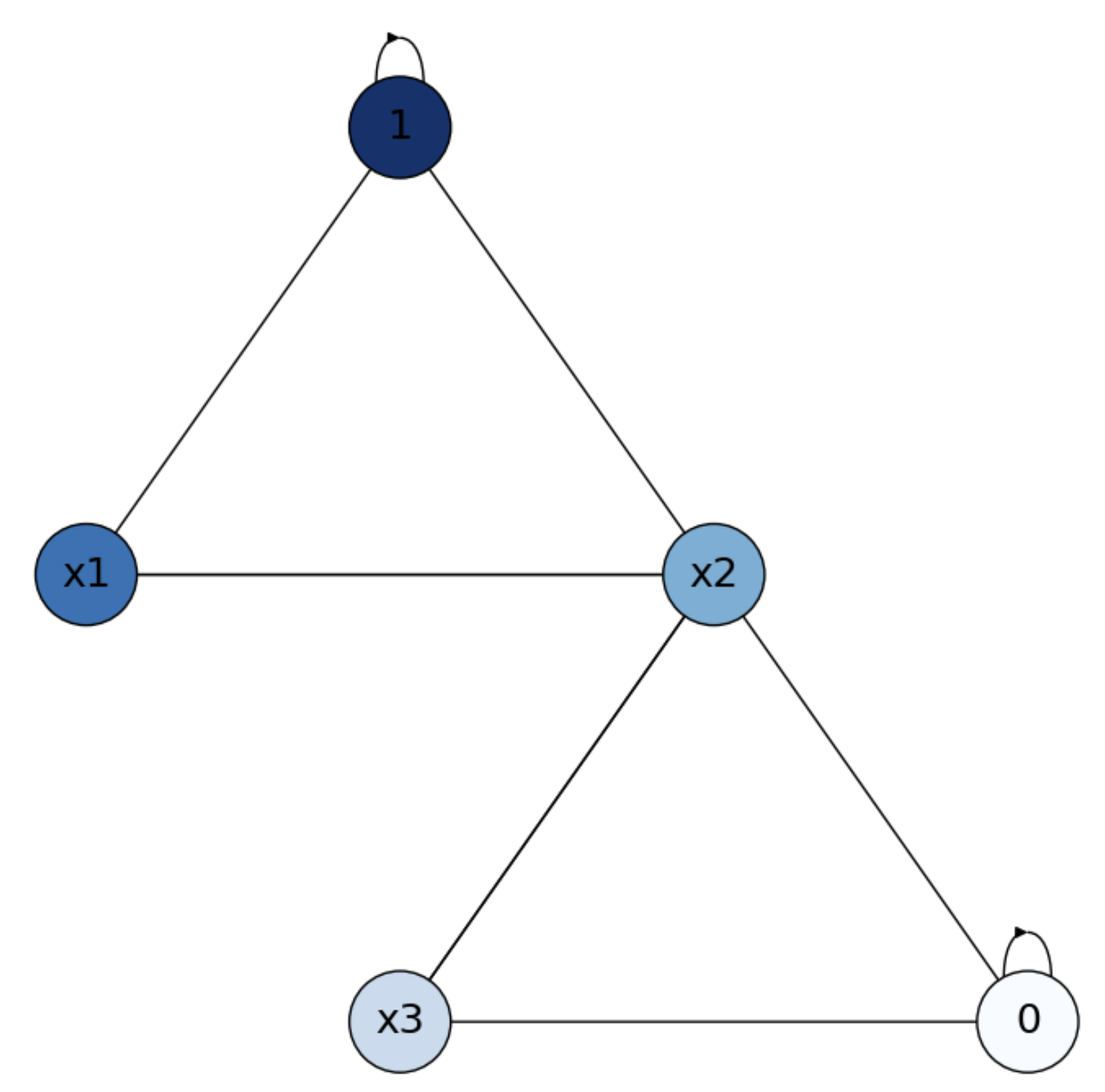
Fig. 21.2 Solution for Triangular mesh with interior nodes \(x_1\),\(x_2\) and \(x_3\).#