3. Probability#
Pierre Simon (Marquis of Laplace) in A Philoshopical Essay on Probabilities comments:
Present events are connected with preceding ones by a tie based upon the evident principle that a thing cannot occur without a cause which produces it.
This leads us directly to “chance”, i.e. we are talking about the “likelihood” of an event in the future based on the present knowledge (also quoting The Feynmann Lectures on Physics).
Actually, probability can be described as the quantification of chance. In discrete probability we talk about a set \(\Omega\) (the sample set) containing all the possible atomic events. Some examples:
\( \begin{align} \Omega_1 &= \{H,T\}\; & \text{Results of tossing a coin: Head (H), Tail (T)}\\ \Omega_2 &= \{1,2,\ldots,6\}\; & \text{Results of playing a dice of 6 faces}\\ \Omega_3 &= \{\omega_1,\ldots,\omega_{52!}\} & \text{Ways of shuffling a standard deck of 52 cards}\\ \Omega_4 &= \{\omega_1,\ldots,\omega_{N_{mn}}\} & \text{Number of paths in a grid}\\ \end{align} \)
Note that sometimes we can explicitly name the atomic events but some other times we can only enumerate how many of them do we have. Anyway, in discrete probability we are always playing with countings.
Actually, the probability of a particular event is the ratio between two counts:
The number of favorable cases (to that event).
The number of all cases.
For atomic events, their probability is simply \(1/|\Omega|\). However, an event is any proposition that can be evaluated to true or false with a certain probability, such as: “playing a dice returns an even value with probability \(3/6\)”. In this case, the event “even” is not atomic, but a subset \(A\subseteq \Omega\), where \(A=\{2,4,6\}\), i.e. the elements in \(\Omega\) that satisfy the logical proposition “return an even value”. We formalize this as follows:
Axioms of Probability. Given an atomic event \(\omega\in\Omega\), its probability \(p(\omega)\) is a function \(p:\Omega\rightarrow [0,1]\) satisfying:
\( 0\le p(\omega)\le 1\; \text{and}\; \sum_{\omega\in\Omega}p(\omega) = 1\;. \)
In addition for non-atomic events \(A\) we have:
\( p(A) = \sum_{\omega\in A} p(\omega)= \sum_{\omega\in \Omega} p(\omega)[\omega\in A]\;, \)
where \(p(\omega)[\omega\in A]\) reads: \(p(\omega)\) if \(\omega \in A\) and \(0\) otherwise.
Finally, for a countable sequence of disjoint events \(A_1,A_2,\ldots\) we have the following axiom:
\( p\left(\bigcup_{i=1}^{\infty} A_i\right) = \sum_{i=1}^{\infty} p\left(A_i\right)\;. \)
which is a consequence of the PEI. Actually, if the events are not disjoint we have to consider the full definition of the PEI (excluding-including interesections).
More properties. As a result of the aforementioned axioms, we have:
\( p(\emptyset) = 0\; \text{and}\; p(\Omega) = 1\;. \)
However, \(\emptyset\) may be not the only event with probability zero. Actually:
\( p(\bar{A}) = 1 - p(A)\; \text{(complement)}\; \text{and}\; A\subseteq B\Rightarrow p(A)\le p(B)\;\text{(monotonicity)}\; \)
Finally, we have the binary PEI:
\( p(A\cup B) = p(A) + p(B) - p(A\cap B)\;. \)
3.1. Independent Trials#
3.1.1. Coins and dices#
Events can be seen as the output of a given experiment. One of the most simplest experiments is tossing a coin. There are two possible outputs \(\Omega=\{H,T\}\). If the coin is fair, each of these outputs is equiprobable or equally likely to happen: \(p(H) = p(T) = 1/2\).
Now assume that the coin experiment can be repeated \(n\) times under the same conditions. Each of these repetitions is called a trial. So, a natural question to answer is ”what is the probability of obtaining, say \(k\) heads after \(n\) trials?”. We can use combinatory to answer to this question. Actually, the solution is:
The number of total cases is \(2^n\). If we assign \(1\) to \(H\) and \(0\) to \(T\), we have \(2^n\) possible numbers of \(n\) bits (permutations with repetition) and each of these numbers concatentates the results of \(n\) trials. In addition, only \({n\choose k}\) cases are favorable since we have \({n\choose k}\) groups of \(k\) heads in \(n\) trials.
Actually, we can better understand the above rationale by reformulating \(P(n,k)\) as:
This means that the probability of any trial is \(1/2\) and all the \(n\) trials are independent. Intuitively, statistical independence means that a trial does not influence the following one (same experimental conditions for any trial). More formally, \(n\) events \(A_1, A_2,\ldots, A_n\) are independent if
Then, the probability of obtaining a given sequence say \(HHHTT\) (\(n=5\)) is
Actually, all sequences with \(n=5\) are equiprobable. However, what makes \(HHHTT\) different from the others is the fact that we have \(3\) \(H\)s (and consequently \(5-3=2\) heads). If we want to highlight this fact, we should group all sequences of \(n=5\) trials having \(3\) \(H\)s (or equivalently \(2\) \(T\)s). Some hints:
Order matters. Strictly speaking, sequences such as \(HHHTT\) and \(TTHHH\) should count twice. Since \(H\) and \(T\) can be repeated (three times and twice respectively). we have permutations with repetition:
However, we know that
This is where the combinations come from: we have \(n=5\) positions and we need to fill \(3\) of them (order does not matter) with heads. Then, we have \({5\choose 3}\) ways of doing it. It works because the strings \(11100\) and \(00111\) represent different subsets of \(\{0,1\}^{5}\) and what combinations do is to encode subsets (members of the power set).
Therefore, we have used the product rule to decompose the problem in two parts:
Compute the probability of a configuration: \(p(HHHTT)\).
Compute how many different configurations do you have: \({5\choose 3}\).
Then, the probability \(p(\#H=3,5)\) of having \(3\) heads in \(5\) trials is:
In practice, use permutations with repetitions instead of combinations when the outcomes of a experiment are more than \(2\). We illustrate this case in the following exercise.
Exercise. Consider the problem of throwing a dice \(n=6\) dices simultaneously. What is the probability of obtaining different results? And all equal?
This is equivalent to \(n\) independent dice trials. Since \(|\Omega|=6\), we have that \(p(i)=1/6\) for \(i=1,2,\ldots,6\). Therefore, the probability of a given sequence of \(n\) trials is \((1/6)^n\). This is the first factor of the product rule (the probability of a given configuration).
The second factor (the number of possible configurations) comes from realizing that each of the \(n\) positions can be filled by different values. Since order matters, we have to count the number of permutations without repetition or permutations with individual repetition (the elements must be different) of \(n\) elements. This leads to \(n!\) and
\(
p(\text{All_diff.}) = n!\frac{1}{6^n} = \frac{n!}{1!1!1!1!1!1!}\cdot\frac{1}{6^n}= \frac{6!}{6^6} =\frac{6}{6}\cdot\frac{5}{6}\cdot\frac{4}{6}\cdot\frac{3}{6}\cdot\frac{2}{6}\cdot\frac{1}{6} = 0.015\;.
\)
However, there are \(n=6\) configurations where all the dices give the same result:
\(
p(\text{All_equal.}) = \frac{n}{6^n} = \frac{1}{6^5} = 0.0001\;.
\)
3.1.2. The Binomial distribution#
3.1.2.1. Unimodality#
As we have seen in the previous section, when performing \(n\) independent trials, the odds of some events are higher that those of others. In particular, extremal events \(E\) such as maximizing (or minimizing) the appearance of one of the elements of \(\Omega\) have the smallest probability. However, since the probabilities of all events add \(1\), the bulk of the probability mass should lie in non-extremal events.
In order to see that, we revisite coin tossing, where the two extremal events are \(E=\{\text{All_}Ts, \text{All_}Hs\}\), both with probability \(1/2^n\). Then, we have
As a result, the probability of non-extremal events becomes almost \(1\) as \(n\) grows since:
Being all the particular configurations equiprobable (i.e. \(1/2^n\)), the fact that \(\lim_{n\rightarrow\infty}P(\bar{E}) = 1\) is due to the number that each particular configuration is repeated.
A closer look to \(2^n = {n\choose 0} + {n\choose 1} + {n\choose 2} + \ldots + {n\choose n}\) gives us the answer. The probability of having \(k\) \(H\)s becomes:
and due to the symmetry of \({n\choose k} = {n\choose n-k}\), this probability is going to grow from \(k=0\) until a given \(k=k_{max}\) and then decrease for \(k=n\). Actually:
If \(n\) is even, \(k_{max} = \frac{n}{2}\) and \({n\choose 0}<{n\choose 1}<\ldots <{n\choose \frac{n}{2}}>{n\choose \frac{n}{2}+1}>\ldots>{n\choose n}\).
If \(n\) is odd, \(k_{max} = \frac{n-1}{2}=\frac{n+1}{2}\) and \({n\choose 0}<{n\choose 1}<\ldots <{n\choose \frac{n-1}{2}}={n\choose \frac{n+1}{2}}>{n\choose \frac{n}{2}+1}>\ldots>{n\choose n}\).
That is, for \(n\) odd we have a double maximum of probability. Anyway the distribution of probability among the values \(k=0,1,\ldots,n\) is unimodal. In addition, the increase of probability from \(k-1\) to \(k\) before the maximum is given by
i.e.
These properties can be better understood by studying the Pascal’s triangle.
3.1.2.2. Pascal’s Triangle#
The Pascal’s Triangle has had many names along the history of mathematics (e.g. Tartaglia Triangle). This construction gives the \({n\choose k}\) for all \(n\). For instance, in HT, each column denotes a value of \(n\) and the coefficients in this column are the \(n+1\) so called binomial coefficients for such \(n\): \({n\choose 0},{n\choose 1},\ldots, {n\choose n}\).
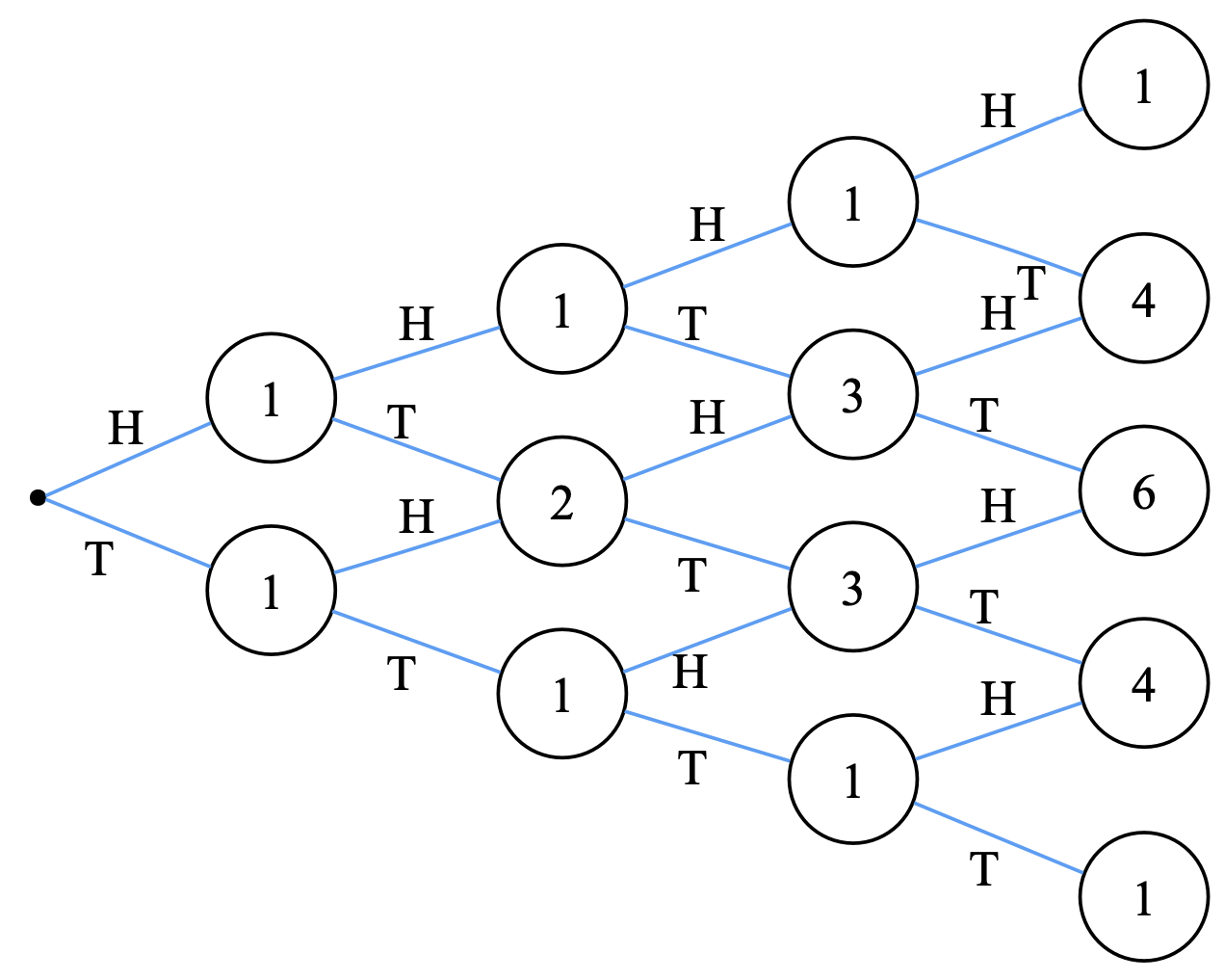
Fig. 3.1 Binomial coefficients.#
The triangle is constructed as follows:
Start by \(n=0\) and make a trial. We have \({1\choose 0}=1\) ways of obtaining a \(H\) and \({1\choose 1}=1\) ways of getting a \(T\). Then set \(n=1\).
From \(H\) we have again \(1\) way of getting a H and one way of getting a \(T\). However, this also happens from \(T\). Therefore, after the second experiment we have \(4\) possible outcomes: \(HH, HT, TH, TT\). Two of these outcomes are extreme event and two of them collapse in the same representation \(HT,TH\) (two ways of getting one \(H\) and one \(T\)). This is way the central node has a value \(2\).
Then, we set \(n=2\) and continue…
Some properties:
As noted above, even columns do have a unique maximual coefficients, whereas odd columns have two.
If the normalize the \(n-\)th column by \(2^n\) we have the discrete probability distribution asociated to having \(k=0,1,2,\ldots,n\) heads \(H\)s.
Extreme events are always placed (by symmetry) in the main diagonals.
Non-extreme or regular events begin to fill the distributions as \(n\) increases.
The coefficients of any regular event can be obtained by adding those of their parents in the tree, since:
The binomial coefficient in a node gives the number of paths that reach that node from the origin (equivalent to \(\#\Gamma\) in a grid without obstacles). We will come back to this fact later on.
As \(n\) increases, it becomes more and more clear that the Binomial probability distribution is centered on \(n/2\), where the probability is maximal and then decreases to two tails corresponding to the extremal events. This allows us to intuitively understand the concept of mean value, as we will define later on.
See for instance Bern, where we highlight the binomial coefficients after \(n=8\) trials. Check that the highest coefficient at level \(n=8\) is at position \(n/2\) (starting by \(0\)).
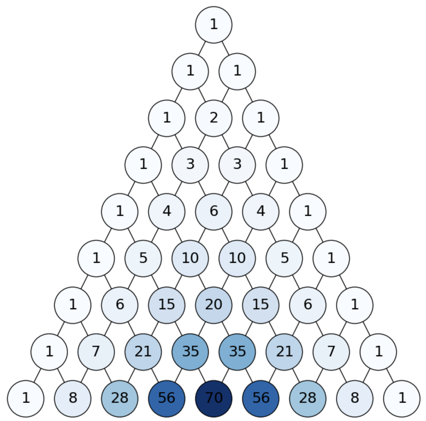
Fig. 3.2 Binomial coefficients.#
Let us express all these things in probabilistic terms!
3.1.2.3. Probable values and fluctuations#
One of the magic elements behind the Pascal’s triangle is that it provides the binomial coefficients, independently of whether we have a fair coin or not.
The fair coin is a particular case where the probability of success in an independent trial (called Bernouilli trial) is \(p=1/2\) (herein, we understand success as “landing on a head”). Consequently, the probability of failure (“landing on a tail”) is \(q = 1 - p = 1/2\). Then, the probability of \(k\) successes after \(n\) trials is more generally given by
Then, \(P(n,k)\) is the probability of having \(k\) successes out of \(n\) trials. This is the solid line in PD, where we have performed \(10,000\) games, each one with \(n=1,000\) and \(p=1/2\). In the \(x\) axis we place \(k=0,1,\ldots,n\) (the leaves in Bern for \(n=1,000\)). In the \(y\) axis we plot (solid line) the theoretical \(P(n,k)\) vales. But we also plot (idealy) a bar per \(k\) value. The height of the bars is similar to \(P(n,k)\) but it is not identical. Why? Because we have performed \(10,000\) games. The height of bar \(k\) \(\times\) \(10,000\) is the number of games where we have obtained \(k\) heads out of \(n=1,000\) trials. This number (called the observed number of successes) is close to \(10,000\cdot P(n,k)\) but it fluctuates around it(sometimes it is larger and sometimes it is lower).
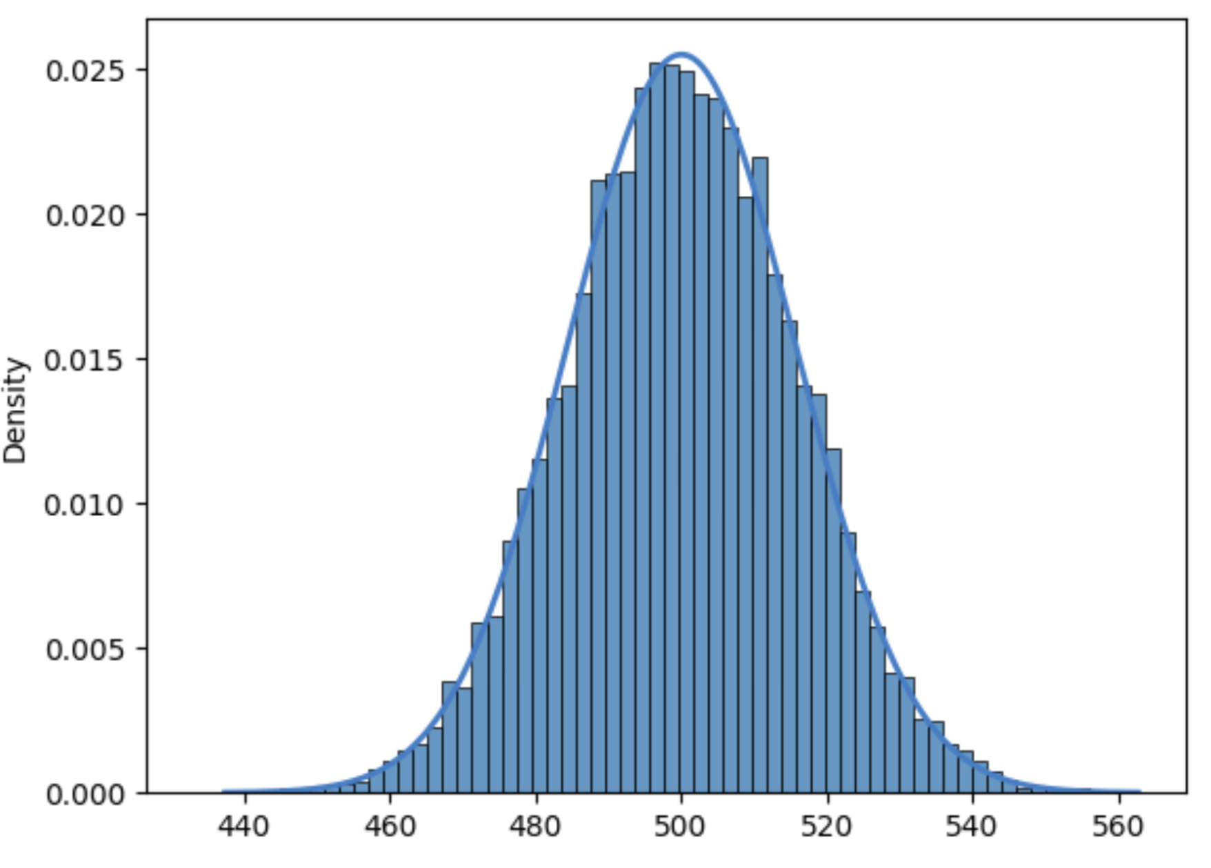
Fig. 3.3 Theoretical probability vs fluctuations.#
Obviously, the most likely or most probable value of \(k\) is \(n/2=500\). However, it is not so obvious why the \(k\)s with smallest nonzero \(P(n,k)\) are close to \(440\) and \(560\). Intuitively, this is related to the extremal events, but these values deserve a deeper mathematical interpretation.
3.1.2.4. Expectation and variance#
Random variables. In the above example, each of the \(10,000\) experiments consists of \(n=1,000\) independent trials, each one resulting in landing either in \(H\)s or \(T\)s with probability \(p\). Then the sample space \(\Omega\) is \(\{H,T\}^{n}\). Well, a random variable \(X\) is a function \(X:\Omega\rightarrow\mathbb{R}\): \(X(\omega), \omega\in\Omega\) , such as the number of \(H\)s. This is indicated by \(X(\omega)=k\), and \(X\sim B(n,p)\) indicates that \(X\) follows a Bernouilli or Binomial distribution.
Expectation. The expectation of a random variable \(X\) is defined as follows:
For \(X\sim B(n,p)\), we have:
The Binomial Theorem. Newton’s binomial theorem is behind the Pascal’s triangle and the Binomial distribution. It basically states that the coefficients of expanding \((x+y)^n\), where \(n\) is an integer, are the binomial coefficients \({n\choose k}\), as follows:
Let us observe the theorem for \(n=0,1,2,\ldots.\)
For \(n=0\), we have \((x+y)^0 = {n\choose 0}x^{0-0}y^{0} = 1\).
For \(n=1\), we have \((x+y) = {n\choose 0}x + {n\choose n}y = 1\cdot x + 1\cdot y\).
For \(n=2\), \((x+y)^2 = {n\choose 0}x^2 + {n\choose 1}xy + {n\choose 1}xy + {n\choose n}y^2 = 1\cdot x^2 + 2\cdot xy + 1\cdot y^2\).
For \(n=3\), \((x+y)^3 = {n\choose 0}x^3 + {n\choose 1}x^2y + {n\choose 2}xy^2 + {n\choose 1}xy^2 + {n\choose n}y^3 = 1\cdot x^3 + 3\cdot x^2y + 3\cdot xy^2 + 1\cdot x^3\).
If you observe the coefficients, they are given by the levels \(n=0,1,2,3,\ldots\) of the Pascal’s Triangle! In other words, herein the extremal events are the unit coefficients of \(x^n\) and \(y^n\) respectively. Then, the corresponding \({n\choose k}\) coefficient of \(x^{n-k}y^k\) is just indicating the corresponding product, i.e. how many \(x\)s and how many \(y\)s do we takein each term.
As a result, the way it is built the Pascal’s triangle plays a fundamental role in the inductive proof of the theorem. Simply remind the expression \( {n\choose k} = {n-1\choose k-1} + {n-1\choose k}\;.\).
Anyway, coming back to the expectation of \(E(X) = np\), just apply the theorem expressing \(p^{r}(1-p)^{(n-1)-r}\) as \(p^{r}q^{(n-1)-r}\) for the binomial coefficient \({n-1\choose r}\). All we are doing is computing \((x+y)^{n-1}\) where \(x+y = p + q = 1\). As a result:
Variance. The fact that when \(X\sim B(n,p)\) we have \(E(X)=np\) gives us directly the most likely number of successes (see PD). However, to explain the amount of deviation from the expectation we rely on the variance which is defined as follows:
In this way, \(Var(X)\) is the expectation of the square deviations from \(E(X)\):
One interesting (and simple) way to compute \(Var(X)\) for Binomial variables \(X\) is to realize that \(X\sim B(n,p)\) means that \(X = \sum_{i=1}^nY_n\) where \(Y_i\sim Bern(p)\),i.e. Bernouilli variables where the outcomes can be \(1\) (success) or \(0\) (failure).
In particular, if \(Y\sim Bern(p)\) we have:
Since \(X\) is the sum of \(n\) \(Y_i\)s: \(E(X) = E(Y_1)+ E(Y_2)+ \ldots + E(Y_n)\). As the expectation of a sum is the sum of expectations (indepedently of whether the variables are independent or not), we have:
Now, for computing \(E(Y^2)\), \(Y\sim Bern(p)\), we do:
As a result
Now exploit the fact that the variance of the sum is the sum of variances when the variables are independent. As this is the case for \(Y_i\sim Bern(p)\). Then we can calculate
It is obvious that \(Var(X)\) increases linearly with \(n\). This simply means that the shape of the distribution (see PD) becomes wider and wider as \(n\) increases? Not really, it is the variance what increases. Later, we will see that for \(n\rightarrow\infty\) we have a Gaussian distribution.
Exercise. It is important to realize that binomial variables are actually sums of Bernouilli trials. But, what can be really considered as a Bernouilli trial? In principle a Bernouilli trial concerns any experiment whose outcome can be grouped into two mutually-exclusive groups: “red vs black”, “red vs (black or green), “even vs odd”, “\(x\le k\) vs \(x>k\)”, etc.
Consider for instance the following Bernouilli trial: Throw \(2\) dices simultaneously and register the outcomes as \((x,y)\). Then infer \(p + q = 1\) in the following cases:
\(
\begin{align}
\;\;\text{a)}\;\; p &= \{\text{Prob. of}\;\; x+y \;\;\text{is even}\}\\
\;\;\text{b)}\;\; p &= \{\text{Prob. of}\;\; x\times y \;\;\text{is even}\}\\
\;\;\text{c)}\;\; p &= \{\text{Prob. of}\;\; x+y>7 \;\;\text{is even}\}\\
\end{align}
\)
and give also the expectations and variances of the Bernouilli variables associated with these experiments.
Firstly, the sample space \(\Omega\) is given by the cartesian product \(\Omega = \{1,\ldots,6\}\times \{1,\ldots,6\}\). Thus, we have
\(
\Omega = \begin{matrix}
(1,1) & (1,2) & (1,3) & (1,4) & (1,5) & (1,6) \\
(2,1) & (2,2) & (2,3) & (2,4) & (2,5) & (2,6) \\
(3,1) & (3,2) & (3,3) & (3,4) & (3,5) & (3,6) \\
(4,1) & (4,2) & (4,3) & (4,4) & (4,5) & (4,6) \\
(5,1) & (5,2) & (5,3) & (5,4) & (5,5) & (5,6) \\
(6,1) & (6,2) & (6,3) & (6,4) & (6,5) & (6,6) \\
\end{matrix}
\)
\(
\Omega_{+} = \begin{matrix}
2 & 3 & 4 & 5 & 6 & 7\\
3 & 4 & 5 & 6 & 7 & 8\\
4 & 5 & 6 & 7 & 8 & 9\\
5 & 6 & 7 & 8 & 9 & 10\\
6 & 7 & 8 & 9 & 10 & 11\\
7 & 8 & 9 & 10 & 11 & 12\\
\end{matrix}
\)
\(
\Omega_{\times} = \begin{matrix}
1 & 2 & 3 & 4 & 5 & 6\\
2 & 4 & 6 & 8 & 10 & 12\\
3 & 6 & 9 & 12 & 15 & 18\\
4 & 8 & 12 & 16 & 20 & 24\\
5 & 10 & 15 & 20 & 25 & 30\\
6 & 12 & 18 & 24 & 30 & 36\\
\end{matrix}
\)
where \(\Omega_{+}\) and \(\Omega_{\times}\) are the sample spaces for the random variables \(X=\{x+y: (x,y)\}\) and \(Y=\{x\times y: (x,y)\}\).
a) For each row in \(\Omega_{+}\) we have \(3\) even and \(3\) odds. As a result, \(p=q=1/2\). Then
\(
\begin{align}
&\;E(X_{even}) = 1\cdot p + 0\cdot q = p = \frac{1}{2}\\
& Var(X_{even}) = E(X_{even}^2) - E(X_{even})^2 = p - p^2 = p(1-p) = pq = \frac{1}{2}\cdot\frac{1}{2} = \frac{1}{4}
\end{align}
\)
b) The odd rows of \(\Omega_{\times}\) have \(3\) even and \(3\) odd. However, the even rows have \(6\) (all) even and \(0\) (none) odd. As a result, we have \(3\times 3 + 3\times 0 = 9\) odd outcomes and \(3\times 3 + 3\times 6 = 27\) of \(36\) outcomes. Then, we have \(p = 27/36 = 3/4\) and \(q = 9/36 = 1/4\). Then
\(
\begin{align}
&\;E(Y_{even}) = 1\cdot p + 0\cdot q = p = \frac{3}{4}\\
& Var(Y_{even}) = E(Y_{even}^2) - E(Y_{even})^2 = p - p^2 = p(1-p) = pq = \frac{3}{4}\cdot\frac{1}{4} = \frac{3}{16} = 0.1875
\end{align}
\)
c) For this part we need to compute the domain of \(X=\{x+y: (x,y)\}\), which is \(X=\{2,3,\ldots,12\}\). We also need to know the frequencies of each value. The frequencies of the sums are given by the symmetries of this operator:
\(
\begin{align}
X(2) &=X(1,1)=1\\
X(3) &=X(1,2)=X(2,1)=2\\
X(4) &=X(1,3)=X(3,1)=X(2,2)=3\\
X(5) &=X(1,4)=X(4,1)=X(2,3)=X(3,2)=4\\
X(6) &=X(1,5)=X(5,1)=X(2,4)=X(4,2)=X(3,3)=5\\
X(7) &=X(1,6)=X(6,1)=X(2,5)=X(5,2)=X(3,4)=X(4,3)=6\\
X(8) &=X(2,6)=X(6,2)=X(3,5)=X(5,3)=X(4,4)=5\\
X(9) &=X(5,4)=X(4,5)=X(6,3)=X(3,6)=4\\
X(10) &= X(6,4)=X(4,6)=X(5,5)=3\\
X(11) &=X(6,5)=X(5,6)=2\\
X(12) &=X(6,6)=1\\
\end{align}
\)
Then, \(Z_{x+y>7}\) has \(5+4+3+2+1 = n(n+1)/2 = 5\cdot (5+1)/2 = 15\) favorable outcomes out of \(36\) possibilities. As a result, we have \(p = 15/36=5/12\) and \(q = 21/36 = 7/12\). Then
\(
\begin{align}
&\;E(Z_{x+y>7}) = 1\cdot p + 0\cdot q = p = \frac{5}{12}=0.42\\
& Var(Z_{x+y>7}) = E(Z_{x+y>7}^2) - E(Z_{x+y>7})^2 = p - p^2 = p(1-p) = pq = \frac{15}{36}\cdot\frac{21}{36} = 0.24
\end{align}
\)
3.1.2.5. Fundamental inequalities#
Extremal events have small probabilities. In \(X\sim B(n,p)\) the probability decays from its maximum value (for \(k=\lfloor np\rfloor\)) until close-to-zero at the extremal events. Such a decay is somewhat described by \(Var(X)\). However, we have to go deeper in order to characterize the probability of rare events.
Firstly, we should measure how the probability decays as we move away from the expectation. For this task, we rely again on looking \(X\sim B(n,p)\) as the sum of \(n\) Bernoulli trials \(Y_i\sim Bern(p)\).
For \(X = Y_1 + Y_2 + \ldots Y_n\), we have
Hoeffding’s theorem bounds \(p(X - E(X)\ge t)\) for \(t>0\) and \(X\) being the sum of \(n\) independent variables \(Y_i\) satisfying \(a_i\le Y_i\le b_i\) almost surely or a.s. (i.e. with probability \(1\)), as follows:
This theorem, simply means that deviating \(t\) units from \(E(X)\), results in an exponential decay. This justifies the exponetial shape of the Binomial distribution as we move from \(E(X)\) towards the extremal events! In particular, for this distribution, where \(0\le Y_i\le 1\) a.s., the Hoeffding’s bounds are:
Interestingly, the exponential decay is attenuated by \(n\): the larger \(n\) the slower the decay since the distribution becomes flatter and flatter as \(n\) increases.
Cumulative distribution. So far, we have been focused on describing random variables in terms of characterizing \(p(X=x)\) (point-mass function or pmf). However, sometimes it is useful to quantify the bulk of the probability, for instance between two extremal values \(a<b\). For \(X\sim B(n,p)\), we now that this bulk is almost \(1\) (but not almost sure unless \(n\rightarrow 1\), since extremal events exist). However, for \(k:a\le k\le b\), what is the probability that the number of heads is “less or equal than k”?
The usual way to answer this question is to calculate \(p(X\le k)\):
We can use the Hoeffding’s bound to give an idea of this probability, since
Actually, \(p(X\le k)\) is much larger that the neg-exp. Interestingly, when \(k\approx np\) (close to the expected value), \(p(X\le k)\ge \frac{1}{n}\), but actually it is \(p(X\le np)=1/2\) due to the symmetry of the distribution. Therefore, the Hoeffding’s bound is a very conservative bound.
The Chernoff bound is one of the tighest bounds for quantifying the probability of rare events. It is formulated as follows. If we have \(n\) independent variables \(Y_1,Y_2,\ldots, Y_n\) with \(p(Y_i=1)=p_i\) and \(p(Y_i=0)=1-p_i\), \(X = \sum_{i=1}^nY_i\) has expectation \(E(X) = \sum_{i=1}^np_i\) and we have:
The above formulation of the Chernoff bound was proposed in the Survey paper dealing with concetration inequalities. Actually, we have:
The lower tail bound holds for all \(\lambda\in [0, E(X)]\) and hence for all real \(\lambda\ge 0\).
The upper tail bound, too, holds for all real \(\lambda\ge 0\).
Note that this version of the Chernoff bound decays more slowly than the Hoeffding’s bound since the denominator is dominated by \(E(X)\).
Let us now compute the probabilities for the tails in PD: \(440\) and \(560\). Since \(E(X) = np = 500\), we have that \(440-500 = -60\) and \(560 - 500 = 60\), we set \(\lambda = 60\). Then
\(p(X-E(X)\le -\lambda)\le \exp\left(-\frac{60^2}{1000}\right) = 0.0027\).
\(p(X-E(X)\ge \lambda)\le \exp\left(-\frac{60^2}{2(500+60/3)}\right) = 0.0031\).
So far, we have characterized the Binomial distribution (concept, expectation, variance and rare events). The Binomial distribution plays a fundamental role in the analysis of AI algorithms for discovering the best solution (whenever possible). These algorithms explore a tree in an “intelligent way”. Before giving an intution of this point, let us introduce an important concept also related with probability and “exploration”: the random walk. In particular, we will focus at random walks under the Binomial distribution.
3.1.2.6. Random walks#
Let us start by defining the following game:
Put a traveler at \(x=0\).
Toss a coin.
If the result is head move right: \(x = x + 1\).
Otherwise, move left: \(x = x - 1\).
Continue until arriving to \(n\) tosses.
The above procedure describes a one-dimensional random walk through the \(\mathbb{Z}\). One of the purposes of this game is to answer the question: “How far the traveler gets on average?”
A bit formally, the problem consist of finding the expectation of \(Z\), the sum of \(n\) independent events \(Y_i\) with output either \(+1\) or \(-1\). For a fair coin, \(E(Y_i) = 1\cdot p + (-1)\cdot p = 0\) and this implies that \(E(Z)=E(\sum_{i=1}^n Y_i)= \sum_{i=1}^nE(Y_i)=0\).
Actually, under fairness, we can also answer the question: ”What is the probability of landing at a give integer \(z\) after \(n\) steps?”. This can be done by simply quering the Pascal Triangle!
In other words, this problem is equivalent to placing the \(\mathbb{Z}\) line on top on the Pascal’s triangle and aligning \(x=0\) with the top vertex of the triangle. We do that in PascalZ, for clarifying that:
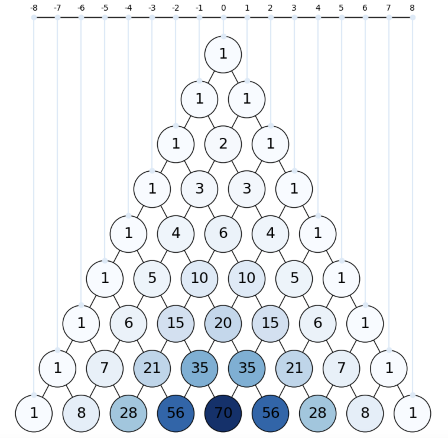
Fig. 3.4 One-dimensional (fair) Random Walk over Pascal’s Triangle.#
The random walker (RW) may progress towards the left (negative), the right (positive) or coming back home (zero). Landing at a given integer \(z\) is just the probability \(P(z,n)\) of \(z\) successes (if \(z>0\)) or failures (if \(z<0\)).
In
PascalZ, we link \(z\in\mathbb{Z}\) with nodes of the respective first levels where we have \(z\) successes (failures), but this line do extend to nodes below them if this property is satisfied: “if we do not have \(z\) successes (failures) yet, maybe we may have them later”. This is basically the gambler’s conflict!However, in the long run it is expected that the gambler lands on \(z=0\) (no win - no lose) if its wealth is large enough. This is because \(E(Z) = 0\) is equivalent to \(E(X)=np\) for \(X\sim B(n,p)\).
Of course, the hope (land on \(z>0\)) or risk (land on \(z<0\)) is measured by the probability of extremal events as we explained above.
Logically, if extremal events do happen much more frequently than when predicted by the theory, one may think that the coin is loaded (not fair).
Regardless of direction. We have seen that \(E(Z) = 0\) (going forward and backwards is equally likely). However, what happens if we reformulate the original question as follows: “How far the traveler gets on average, regardless of direction?”. Answering this question implies computing
Using the identity (for any \(Z\) given by the sum of independent identically distributed or i.i.d. variables):
Hence, we have \(Var(Z) = nVar(Y)\) since the variables \(Y_i\) are i.i.d., so we proceed to measure
Since \(p = q\) for a fair coin, we have \(Var(Y) = 1\) and, a result \(Var(Z)=E(Z^2)=n\). For instance, in RWrand we plot \(100\) fair RWs for \(n=10,000\). The darkness of the blueness of each walk is proportional to \(Var(Z)=E(Z^2)\) (we have inverted this brightness wrt previous figures for better visualizing extremal paths). Note that most of the paths have “deviations” upper bounded by \(\pm 3\sqrt{Var(Z)} = \pm 3\sqrt{n} = \pm 300\).
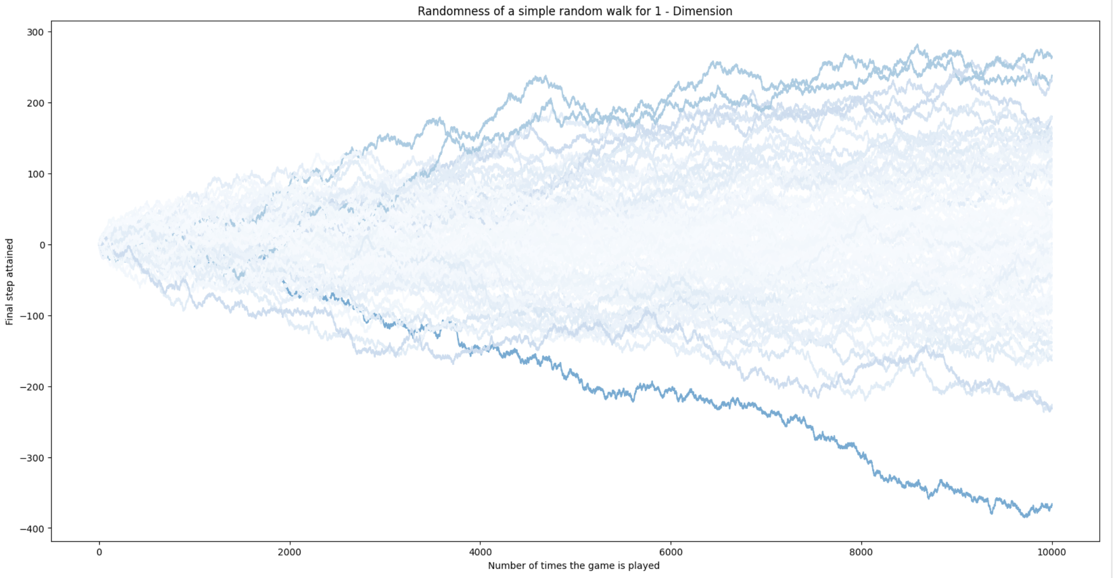
Fig. 3.5 One-dimensional (fair) Random Walk: deviations.#
3.1.2.7. The Normal distribution#
When \(n\rightarrow\infty\), the combinatorial nature of \(B(n,p)\) and its links with random walks can be described in a simpler way. The \(B(n,p)\) in the limit becomes another distribution: the well-known Normal or Gaussian distribution.
In this regard, we exploit the Stirling’s approximation rewriten as
We plug in this formula in the probability of \(k\) successes, in order to approximate all the factorials:
At this point, it is convenient to formulate the number of succeses \(k\) in terms of deviations \(k = np + z\) from the expectation \(np\) as we did when defining random walks. As a result,
and we have
Since
we have
Now, in order to highlight the exponential shape of \(p(X = np + z)\) let us take logs at both sides
Now, we exploit the Taylor expansions of \(\log(1+x) = x - \frac{1}{2}x^2 + \frac{1}{3}x^3\ldots\) and \(\log(1-x) = -x - \frac{1}{2}x^2 - \frac{1}{3}x^3\ldots\)
Taking up to the quadratic terms, for A, B we have
Then, we have
and similarly
Plugging \(A\), \(B\), \(C\) in
As a result, if we replace \(z\) by \(k - pq\) we have
i.e., the so called De Moivre - Laplace theorem yields the usual expression for the Normal distribution as a limit of the Binomial one:
More generally, as \(np\) is the “mean” of the Binomial, it is renamed as mean \(\mu\) of the Normal. Similarly, as \(npq = Var(X)\), it is renamed the variance \(\sigma^2\) of the Normal, whose squere root is the standard deviation \(\sqrt{\sigma^2}=\sigma\).
Therefore, we can say that \(X\sim N(\mu,\sigma^2)\) if its pmf is
The Standarized Normal. Coming back to the fact that
we translate that to
Then, the above definition becomes
However, this expression is not yet a probability mass function but a probability density function pdf since:
It does not yet describe the probability that the RW is at position \(z\), but the probability thast a RW with step-length \(1\) on average is near \(z\).
As a result, \(p(X=z)=0\) since we cannot undo precisely the run of the RW to land at an specific \(z\) but to land at an interval \(\Delta z\). The smaller the \(\Delta z\) (it becomes a differential \(dz\rightarrow 0\)) the more precise is our result (see Feynman Lectures), and this happens when \(n\rightarrow\infty\):
Then, the cumulative distribution becomes:
In particular, let us define the (continuous) random variable \(Z\) where,
Then thr unit or standarized Normal distribution and its pdf is given by
Actually, the above integral, known as the Gauss integral satisfies the axioms of probability since
meaning that the area under the Gauss function defines a probability. In particular, looking at GaussU we have:

Fig. 3.6 Cumulatives of the unit Gaussian: \(a=-1, b=1\).#
Probability of \(Z\le a\) (lower tail):
Probability of \(a\le Z\le b\) (between \(a\) and \(b\)):
Probability of \(Z\ge a\) (upper tail):
Basically, once you standarize a variable \(X\) (i.e. transform it into \(Z\)), you have all you need to compute Gaussian probabilities:
If you want to query the lower tail values, please visit the Standard Normal Cumulative Probability Table
Link with fundamental bounds. Once that we have discovered the exponential nature of the Gaussian, and once we realized that the Gaussian is the limit of the Binomial, we close the loop of understanding the exponential decays of both the Hoeffding’s and Chernoff bounds.
3.2. Statistical dependence#
3.2.1. No replacement#
Assuming that events are iid (independent and identically distributed) is somewhat far from modeling real events. The simplest way of understanding that is change the conditions of the experiment from one trial to another (no replacement).
Take for instance a standard deck of \(52\) cards: \(4\) suits (clubs \(\clubsuit\), diamonds \(\diamondsuit\), spades \(\spadesuit\) and hearts \(\heartsuit\)) and for each of them \(2-10\) cards, plus Ace, \(A\), Jack \(J\), Queen \(Q\) and King \(K\): \(13\times 4 = 52\) cards. In addition,
Diamonds and hearts are \(\text{Red}\), whereas the other two suits are \(\text{Black}\).
Jacks, Queens and Kings are \(\text{Face}\) cards.
Then, the probability of obtaining a spade is \(p(\spadesuit)=\frac{13}{52}=1/4\). However:
If we obtain a \(\spadesuit\), remove it from the deck and shuffle again, the probability changes: \(p(\spadesuit'|\spadesuit)=\frac{12}{51}=0.235<1/4\).
It also changes if we obtain a card of any other suit, say \(\diamondsuit\), but in a different way: \(p(\spadesuit'|\diamondsuit)=\frac{13}{51} = 0.254>1/4\).
In both cases, the notation \(p(A|B)\) denotes the probability of obtaining \(A\) given \(B\). In both cases, the conditioning modifies the probability of the original event \(A\). Therefore, \(A\) is conditionally dependent on \(B\). In other words \(A\) and \(B\) are independent only if
In addition, condititional probability is computed by the Bayes theorem:
Now, enforce not-independence or conditioning (dependence) by drawing \(k\ll 52\) cards without replacement and then asking for the probability of certain events related to these \(k\) cards.
For instance, if we draw two cards sequentially, what is the probability of obtaining an ace of diamonds \(A\diamondsuit\) and a \(\text{Black}\) card.
Since we draw the \(k\) cards sequentially, the we have to consider the \(k!\) possible orders of obtaing \(k\) cards from \(52\). In this case, we have \(k=2\) and consequently two possible orders:
First \(A\diamondsuit\), second \(\text{Black}\).
First \(\text{Black}\), second \(A\diamondsuit\).
We denote the events as follows:
\( \begin{align} A &=\{\text{First card is}\; A\diamondsuit\}\\ B &=\{\text{Second card is}\; A\diamondsuit\}\\ C &=\{\text{First card is}\; \text{Black}\}\\ D &=\{\text{Second card is}\; \text{Black}\}\\ \end{align} \)
Then, we explore the probability of each “order”:
\( \begin{align} p(A\cap D) &= p(A)p(D|A) = \frac{1}{52}\cdot\frac{26}{51} = \frac{1}{102}\\ p(C\cap B) &= p(C)p(B|C) = \frac{26}{52}\cdot\frac{1}{51} = \frac{1}{102}\\ \end{align} \)
Therefore, since both orders are disjoint, the final result is given by
\( p(A\cap D) + p(C\cap B) = \frac{1}{102} + \frac{1}{102} = \frac{2}{102} = \frac{1}{51}\;. \)
Tree diagrams. As we did with coins (\(H\),\(T\)) and the Pascal’s triangle (see HT), representing conditional-probability problems with trees facilitates the visualization of the problem and the interpretability of the solution. Probability trees are built as follows:
The root of the tree is the origin of the experiment.
All the edges are directed and they go from level \(l\) to level \(l+1\). The edges are labeled with probabilities. The edges leaving a given node \(n\) must add the unit.
The edges leaving the root (level \(l=0\)) are associated with non-conditional probabilities of events, e.g. \(p(A)\).
The edges in levels \(l>0\) are associated with probabilities conditioned to the previous level e.g \(p(B|A)\).
The nodes describe events.
The leaves encode intersectional events e.g. \(p(A\cap C)\).
Before using tree diagrams, it is interesting to note that tree diagrams are not well suited for solving problems like the above card-deck problem: what is the probability of obtaining an ace of diamonds \(A\diamondsuit\) and a \(\text{Black}\) card taken sequentially (without replacement). Why?
Take an order, for instance \(A,D\) (first card is \(A\diamondsuit\), second is \(\text{Black}\)). As the probability of the branches must add \(1\), we cannot put \(A\) and \(D\) as branches since \(p(A) + p(D)\neq 1\).
We actually need a tree for each order.
In the first tree, we encode the order \(A,D\) (first card is \(A\diamondsuit\), second is \(\text{Black}\)) to calculate \(p(A)\) and \(p(D|A)\) leading to \(p(A\cap D)\).
In the second tree, we encode the order \(C,B\) (first card is \(\text{Black}\) and second is \(A\diamondsuit\)), to calculate \(p(B)\) and \(p(C|B)\) leading to \(p(C\cap B)\).
In Tree1, we show the first of these two trees. Note that half of the nodes provided answers not required in this particular problem. However, the answer \(p(A\cap D)\) added to that of \(p(C\cap B)\) given by a second tree, solves the problem.
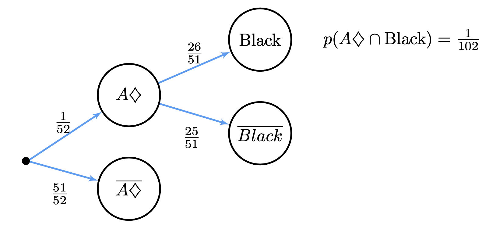
Fig. 3.7 Simple tree for \(p(A\cap D)\).#
Despite the above example, tree diagrams are very useful in other no-replacement problems such as answering the following gambling question:
What is the probability that after extracting two cards from the deck, without replacement, I get two cards with the same color?
We build the tree diagramm as follows:
Level \(1\): we have two possibities \(R = \{\text{1st card is}\; \text{Red}\}\) or \(\bar{R} = \{\text{1st card is}\; \text{Black}\}\).
Level \(2\): we have, again two possibities \(R' = \{\text{2nd card is}\; \text{Red}\}\) or \(\bar{R'} = \{\text{2nd card is}\; \text{Black}\}\).
Then, the probabilities of the two branches at level \(1\) are:
\( \begin{align} p(R) & = \frac{26}{52} = \frac{1}{2}\\ p(\bar{R}) & = 1 - p(R) = 1 - \frac{1}{2} = \frac{1}{2}\\ \end{align} \)
In level \(2\) we have \(4\) branches:
\( \begin{align} p(R'|R) & = \frac{26-1}{52-1} = \frac{25}{51}\\ p(\bar{R'}|R) & = 1 - p(R'|R) = 1 - \frac{25}{51} = \frac{26}{51}\\ p(R'|\bar{R}) & = \frac{26}{52-1} = \frac{26}{51}\\ p(\bar{R'}|\bar{R}) & = 1 - p(R'|\bar{R}) = 1 - \frac{26}{51} = \frac{25}{51}\\ \end{align} \)
which lead to \(4\) intersection probabilities:
\( \begin{align} p(R)p(R'|R) & = \frac{1}{2}\cdot\frac{25}{51} = p(R\cap R')\\ p(R)p(\bar{R'}|R) & = \frac{1}{2}\cdot\frac{26}{51} = p(R\cap \bar{R'})\\ p(\bar{R})p(R'|\bar{R}) & = \frac{1}{2}\cdot\frac{26}{51} = p(\bar{R}\cap R')\\ p(\bar{R})p(\bar{R'}|\bar{R}) & = \frac{1}{2}\cdot\frac{25}{51} = p(\bar{R}\cap \bar{R'})\\ \end{align} \)
As a result, we are interested in events \(R\cap R'\) and \(\bar{R}\cap \bar{R'}\), i.e. the solution to the problem is
\( p(R\cap R') + p(\bar{R}\cap \bar{R'}) = \frac{1}{2}\cdot\frac{25}{51} + \frac{1}{2}\cdot\frac{25}{51} = \frac{25}{51}\;. \)
Basically, when we extract a card of a given color, we reduce the odds of extracting a sample of the same color in the future and increase those of the opposite color. In other words, we are asking the probability of imbalancing the odds. The probability of balancing the odds is actually
\( p(R\cap \bar{R'}) + p(\bar{R}\cap R') = 1 - \left(p(R\cap R') + p(\bar{R}\cap \bar{R'})\right) = \frac{26}{51}\;, \)
i.e. slightly higher than that of imbalancing the odds.
We show the tree diagram in Tree2. Note that at each level \(l\) of the tree we have that the probability of all the leaves adds to one.
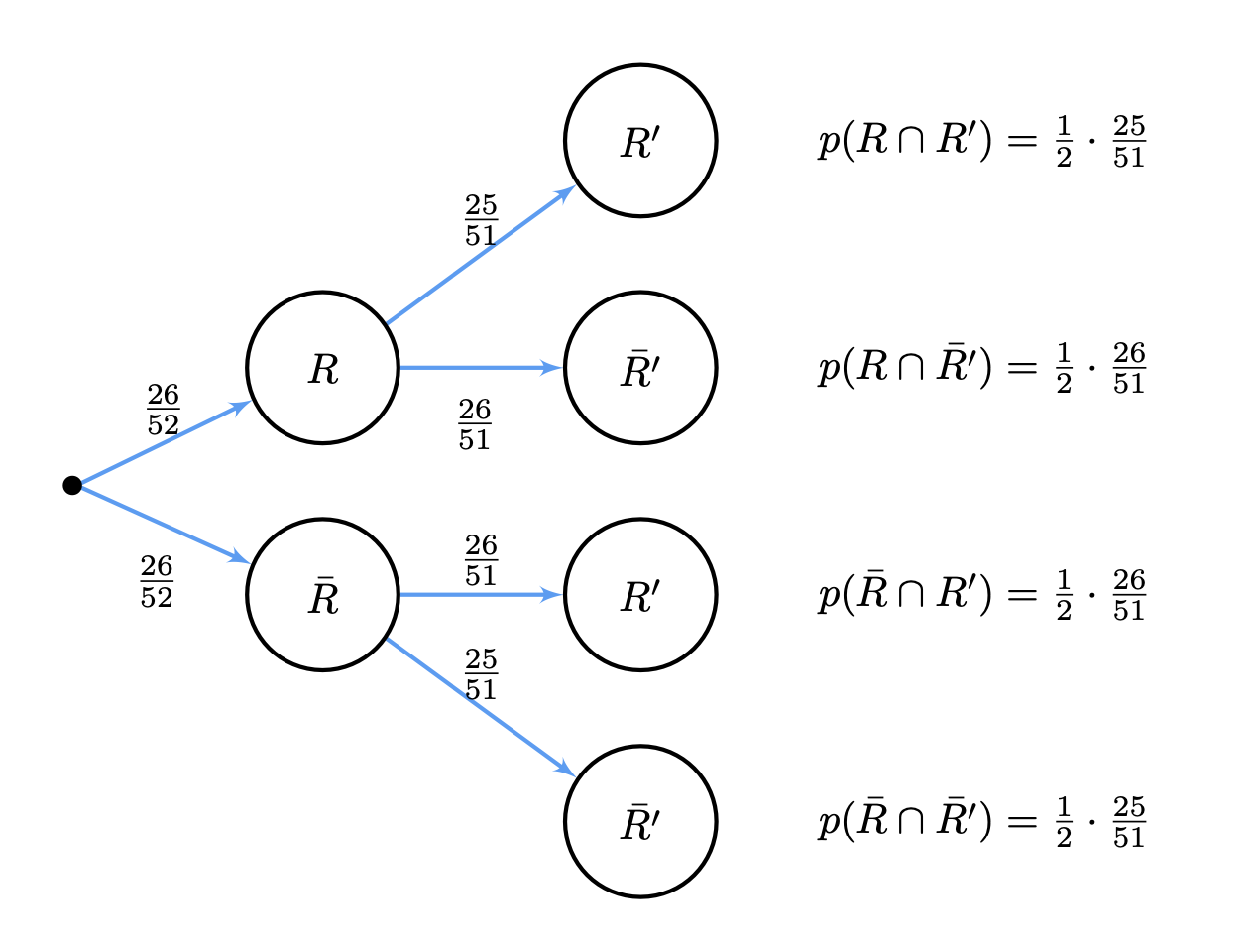
Fig. 3.8 Tree diagram for a card deck (no replacement).#
Note also that \(p(R\cap \bar{R'}) = p(\bar{R}\cap R')\) and the second and third leaves can be fused in just one with probability \(2\frac{1}{2}\cdot\frac{26}{51}=\frac{26}{51}\). Actually, both events represent the same outcome in different orders if consider obtaning a red card a “success” (either in the first or in the second round) and not obtaining it a “failure”.
Therefore, in some regard, this kind of tree remind us the Pascal’s tree, but this time describing conditional events or variables instead of independent ones.
3.2.2. Conditional expectations#
Before we dive deeper in “conditional trees”, it is interesting to redefine expectations in terms of conditional probabilities.
Consider for instance Tree3 where we generalize the tree in Tree2 as follows.
The nodes are considered as the states of a random system with a tuple \((\text{cards},\text{deck})\), where \(\text{cards}\) denote the number of red cards remaining in the deck, and \(\text{deck}\) is the number of cards (both red and black) remaining in the deck.
The edges are labeled with the conditional probability of reaching the destination node from the original one. The probabilities emanating from the same node must add one.
Now, we define the following random variables:
\(X_0=\frac{a}{A}\) is the fraction of red cards in the original deck where:
\(A\) is the number cards in the original deck (\(52\)).
\(a\) is the number of red cards in the deck (\(26\)).
\(X_1\) is the fraction of red cards remaining after the first draw with no replacement.
\(X_2\) is the fraction of red cards remaining after the second draw with no replacement.
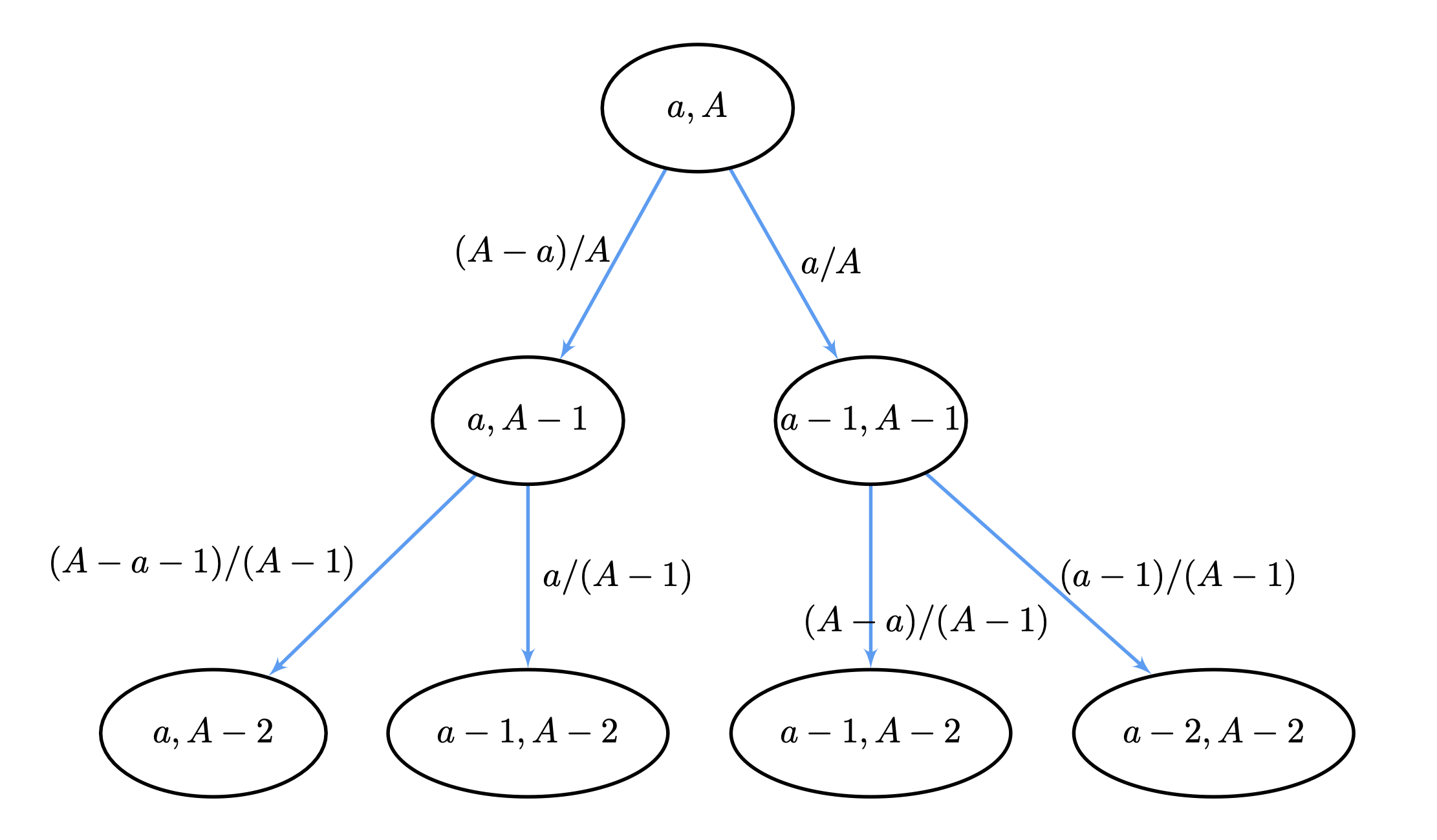
Fig. 3.9 General tree diagram for a card deck (no replacement).#
Then, we define the conditional expectation \(E(X|Y=y)\) of \(X\) wrt to setting \(Y=y\) as follows:
where \(p(X=x,Y=y)\) is the joint probability (intersection).
Consider for instance, \(X=X_1\) and \(Y=X_0\). Since \(X_1\) has two states, we commence by defining the conditional probabilities:
i.e. knowing \(X_0 = \frac{a}{A}\) does not modifies the probability of \(X_1\) (\(X_0\) and \(X_1\) are independent).
Since \(X_0\) has a single value, we have
Since \(X_0\) and \(X_1\) are independent, we have that \(E(X_1|X_0)=E(X_1)\).
However \(X_2\) depends clearly on \(X_1\). Looking at level \(l=2\) we have \(3\) different values for \(X_2\): \(\frac{a}{A-2}\), \(\frac{a-1}{A-2}\) and \(\frac{a-2}{A-2}\).
Let us compute the conditional probabilities for \(X_2\) (actually the probability of each leaf in the tree). Herein, we apply the chain rule for conditional probabilities \(p(X|Y,Z) = p(X|Y)p(Y|Z)\).
Then, looking at the tree we consider the paths leading to each different leaves:
\(X_2 = 0\;\text{red cards extracted}\) (left branch):
\(X_2 = 1\;\text{red card extracted}\) (middle branches):
\(X_2 = 2\;\text{red cards extracted}\) (right branch):
Then, we proceed to calculate \(E(X_2|X_1,X_0)\) as follows:
Look carefully the pattern of the above expression:
We move from \(0\) successes (red card drawn) to \(1\) and \(2\) successes.
Each success is characterized by \(a - k\), with \(k=0,1,2\).
Each failure is characterized by \(A - a - l\), with \(l=0,1\).
Rearranging properly each term so that failures appear first, we have
Therefore, we have that \(E(X_2|X_1,X_0) = E(X_1)\). This property is not satisfied, in general, by any conditional expectation, but when it happens, we say that we have a martingale.
3.2.3. Martingales#
Given a sequence of random variables \(X_0,X_1,\ldots,X_n,X_{n+1}\), it is a martingale if
In the previous example, \(E(X_{n+1}|X_n,\ldots,X_1,X_0)=\frac{a}{A} = E(X_1)\), even if the variables are conditioned.
Why Martingales are useful in Artificial Intelligence?
Martingales are random or stochastic processes not so simpler than sums of i.i.d.s (coin tossing) but not too complex to study. Interestingly, random walks are particular cases of martingales.
The idea behind martingales is that expectation never changes even when you add a new level in the tree (a new conditioned variable). On average, the value of the variable \(X_{n+1}\) is that of \(E(X_{n})\) which does not mean that \(X_{n+1}\) is only conditioned to \(X_{n}\) as it happens in Markov chains. Actually, \(X_{n+1}\) is conditioned to \(X_n,X_{n-1},\ldots,X_0\) but the conditional expectation is invariant.
Fair games. The invariance of the conditional expectation explains the application of Martingales to model the expectations of gamblers in fair games:
Let us define a gambler betting \(1\) coin for the Casino drawing a red card from the deck. If we wins, he gets \(1\) back. Doing so, the expected profit is constant. Why?.
\(X_{n}\) models the gambler fortune at the end of the \(n^{th}\) play.
If the game if fair, the expected fortune \(E(X_{n+1})\) at the game \(n+1\) is the same than that at game \(n\) \(E(X_{n})\), i.e. conditional information cannot predict the future.
3.2.4. Links with Pascal’s Triangle#
Looking carefully at the structure of \(E(X_2|X_1,X_0)\) we have that it is equal to:
where \(p(R_2=k)\) is the probability of drawing \(k\) red cards at level \(l=2\).
In general we have:
where \(P(n,r) = n(n-1)\ldots (n - r + 1)\) is an r-permutation of \(n\) as defined in the topic of combinatorics. The above expression comes from observing the factorial patterns in both the numerator and the denominator.
Compared with the i.i.d. case (Bern), i.e. with replacement, where the probability of obtaining \(k\) red cards should be Binomial
with \(p=1/2\), in PascalMartin we show, with colors, the probability distribution for the conditional case, i.e. for the martingale, where we kept \(\frac{a}
{A} = p\) for being comparable to the independent case.
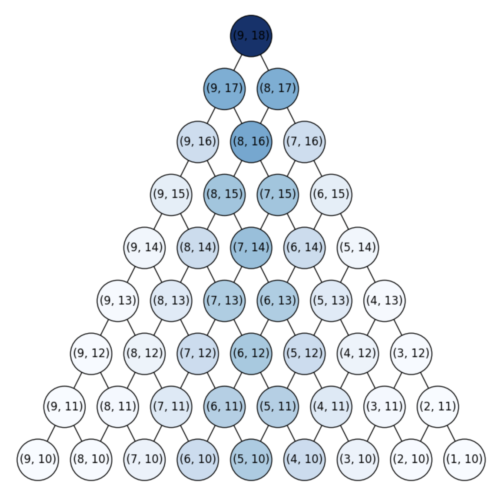
Fig. 3.10 Distribution for a martingale.#
Note that:
Extremal events (all failures/all success) tend to have a zero probability as \(n\) grows.
The bulk of the distribution is close to \(E(X_1)=\frac{a}{A}\) but as \(n\) increases the pmf (point-mass function) is flattened.
Flattening with \(n\) is due to the denominator \(P(A,n)\) of \(p(R_n = k)\).
Of course we may adapt the fundamental equalities defined for i.i.d. variables to conditional ones, but it is quite clear than rare envents will be less probable in conditional trees such as that in
PascalMartinunless we change the ratio between \(a\) and \(A\).