13. Graph Generation

In this section, we will discuss how to generate a graph using the networkx library. Specifically, we will study how to create synthetic graphs, that they are not real-world graphs but are useful for testing and benchmarking algorithms. Also, we will see some important graph properties that can be used to analyze the structure of a graph.

13.1. Synthetic Graphs

A synthetic graph is a graph that is generated artificially, rather than being extracted from real-world data. These graphs are useful for testing and benchmarking algorithms, as they allow us to control the graph’s properties and structure. In this section, we will discuss how to generate synthetic graphs using the networkx library.

13.1.1. Random Graphs

One of the simplest types of synthetic graphs is a random graph. A random graph is a graph in which the edges are generated randomly, subject to certain constraints. There are several models for generating random graphs, such as the Erdős-Rényi model and the Barabási-Albert model.

13.1.1.1. Erdős-Rényi Model

The Erdős-Rényi model is one of the most well-known models for generating random graphs. In this model, we start with a fixed number of nodes and add edges between pairs of nodes with a certain probability. The networkx library provides a function networkx.erdos_renyi_graph to generate random graphs using the Erdős-Rényi model.

import networkx as nx
import matplotlib.pyplot as plt

# Generate a random graph with 10 nodes and edge probability 0.3
G = nx.erdos_renyi_graph(10, 0.3, seed=42)

# Draw the graph
plt.figure(figsize=(6, 6))
plt.title("Random Graph (Erdős-Rényi Model)")
pos = nx.spring_layout(G, seed=42)
nx.draw_networkx_nodes(G, pos, node_size=300, node_color="skyblue")
nx.draw_networkx_edges(G, pos, width=1.0, alpha=0.5)
plt.axis("off")
plt.show()

This code gives us the following graph:

The output of the previous code is the following graph:

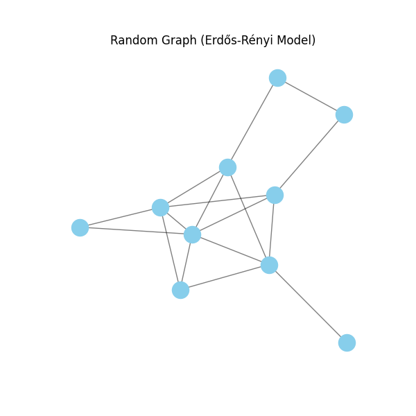
Fig. 13.1 Random Graph (Erdős-Rényi Model)

In the code snippet above, we generate a random graph with 10 nodes and an edge probability of 0.3 using the Erdős-Rényi model. We then visualize the graph using the matplotlib library.

13.1.1.2. Barabási-Albert Model

The Barabási-Albert model is another popular model for generating random graphs. In this model, we start with a small number of nodes and add new nodes with a preferential attachment mechanism, where nodes with higher degrees are more likely to receive new edges. The networkx library provides a function networkx.barabasi_albert_graph to generate random graphs using the Barabási-Albert model.

# Generate a random graph with 10 nodes and preferential attachment parameter m=2
G = nx.barabasi_albert_graph(10, 2, seed=42)

# Draw the graph
plt.figure(figsize=(6, 6))
plt.title("Random Graph (Barabási-Albert Model)")
pos = nx.spring_layout(G, seed=42)
nx.draw_networkx_nodes(G, pos, node_size=300, node_color="skyblue")
nx.draw_networkx_edges(G, pos, width=1.0, alpha=0.5)
plt.axis("off")
plt.show()

This code gives us the following graph:

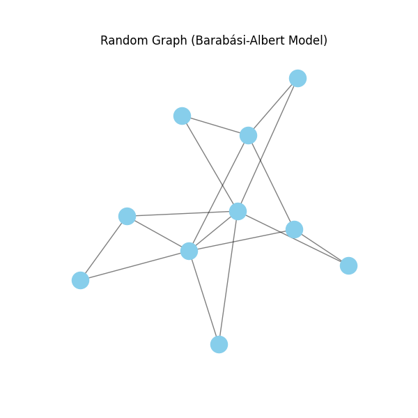
Fig. 13.2 Random Graph (Barabási-Albert Model)

In the code snippet above, we generate a random graph with 10 nodes and a preferential attachment parameter m=2 using the Barabási-Albert model. We then visualize the graph using the matplotlib library.

13.1.2. Small-World Graphs

Another interesting type of synthetic graph is a small-world graph. Small-world graphs are characterized by having a small average shortest path length between nodes, similar to real-world social networks. The networkx library provides a function networkx.watts_strogatz_graph to generate small-world graphs using the Watts-Strogatz model.

# Generate a small-world graph with 10 nodes, average degree 4, and rewiring probability 0.3
G = nx.watts_strogatz_graph(10, 4, 0.3)

# Draw the graph
plt.figure(figsize=(6, 6))
plt.title("Small-World Graph (Watts-Strogatz Model)")
pos = nx.spring_layout(G, seed=42)
nx.draw_networkx_nodes(G, pos, node_size=300, node_color="skyblue")
nx.draw_networkx_edges(G, pos, width=1.0, alpha=0.5)
plt.axis("off")
plt.show()

This code gives us the following graph:

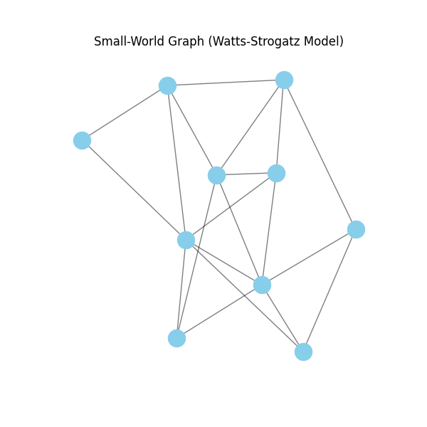
Fig. 13.3 Small-World Graph (Watts-Strogatz Model)

In the code snippet above, we generate a small-world graph with 10 nodes, an average degree of 4, and a rewiring probability of 0.3 using the Watts-Strogatz model. We then visualize the graph using the matplotlib library.

13.1.3. Tree Graphs

A tree is a connected acyclic graph, meaning that there are no cycles in the graph. Trees are a fundamental data structure in computer science and are used in various algorithms and data structures. The networkx library provides a function networkx.random_tree to generate random tree graphs.

# Generate a random tree graph with 10 nodes
G = nx.random_tree(10, seed=42)

# Draw the graph
plt.figure(figsize=(6, 6))
plt.title("Random Tree Graph")
pos = nx.spring_layout(G, seed=42)
nx.draw_networkx_nodes(G, pos, node_size=300, node_color="skyblue")
nx.draw_networkx_edges(G, pos, width=1.0, alpha=0.5)
plt.axis("off")
plt.show()

This code gives us the following graph:

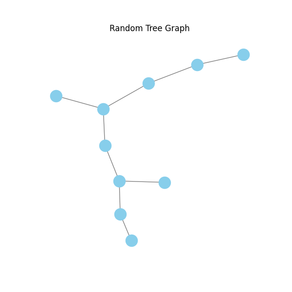
Fig. 13.4 Random Tree Graph

In the code snippet above, we generate a random tree graph with 10 nodes using the networkx.random_tree function. We then visualize the graph using the matplotlib library.

13.1.4. Stochastic Block Model

The stochastic block model is a generative model for random graphs that captures the community structure of the graph. In this model, nodes are divided into blocks or communities, and edges are generated between nodes based on the block they belong to. The networkx library provides a function networkx.stochastic_block_model to generate random graphs using the stochastic block model.

# Generate a random graph with 2 blocks of 20 nodes each
G = nx.stochastic_block_model([20, 20], [
                                            [0.3, 0.01],
                                             [0.01, 0.3]
                                        
                                        ], seed=42)

# Draw the graph
plt.figure(figsize=(6, 6))
plt.title("Stochastic Block Model")
pos = nx.spring_layout(G, seed=42)
nx.draw_networkx_nodes(G, pos, node_size=300, node_color="skyblue")
nx.draw_networkx_edges(G, pos, width=1.0, alpha=0.5)
plt.axis("off")
plt.show()

This code gives us the following graph:

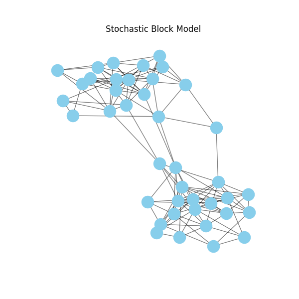
Fig. 13.5 Stochastic Block Model

In the code snippet above, we generate a random graph with 2 blocks of 20 nodes each using the stochastic block model. We then visualize the graph using the matplotlib library.

13.2. Graph Properties

Once we have generated a graph, we can analyze its properties to gain insights into its structure. Some important graph properties that can be computed using the networkx library include:

• Number of Nodes and Edges: The number of nodes and edges in a graph can be computed using the networkx.number_of_nodes and networkx.number_of_edges functions, respectively.

• Is Connected: A graph is connected if there is a path between every pair of nodes in the graph. We can check if a graph is connected using the networkx.is_connected function.

• Does Not Have Cycles: A graph is acyclic if it does not contain any cycles. We can check if a graph is acyclic using the networkx.is_directed_acyclic_graph function.

• Radius and Diameter: The radius of a graph is the minimum eccentricity of any node in the graph, while the diameter is the maximum eccentricity of any node in the graph. We can compute the radius and diameter using the networkx.radius and networkx.diameter functions, respectively. Note that eccentricity is the maximum distance between a node and all other nodes in the graph. Also, this function only works for connected graphs.

• Average Degree: The average degree of a graph is the average number of edges incident to each node in the graph. We can compute the average degree using the networkx.average_degree_connectivity function.

• Degree Distribution: The degree distribution of a graph is the probability distribution of the degrees of the nodes in the graph. We can compute the degree distribution using the networkx.degree_histogram function.

• Average Shortest Path Length: The average shortest path length of a graph is the average distance between pairs of nodes in the graph. We can compute the average shortest path length using the networkx.average_shortest_path_length function.

13.3. Conclusion

In this section, we have discussed how to generate synthetic graphs using the networkx library. We have explored different models for generating random graphs, such as the Erdős-Rényi model, the Barabási-Albert model, and the Watts-Strogatz model. We have also seen how to generate tree graphs and stochastic block model graphs. Finally, we have discussed some important graph properties that can be computed using the networkx library. These properties can help us analyze the structure of a graph and gain insights into its properties.

13.4. Exercises

13.4.1. Exercise 1

After reading the previous section, you should be able to create your first Jupyter-Notebook and write a report about all the things you have learned in this section. In order to have a good structure, we recommend you to follow exactly the same structure as in this notebook.

13.4.2. Exercise 2

Note

NO PUEDE ESTAR DESCONECTADO EL GRAFO. USAR LA MISMA POS PARA EL DRAW, SI NO, SE CASTIGARÁ. JUSTIFICACIÓN EXTENSA Y CON SENTIDO. NADA DE COSAS OBVIAS.

Pay attention to  Stochastic Block Model, and try to generate two graph with 4 blocks of 10 nodes each. The first one, must have the lowest probability of connection between blocks, and the second one, the highest probability of connection between blocks. Then try to visualize the graphs and compare them. In the comparation, try to think about the differences in the structure of the graphs in terms of what would happen if the communities were real people and they try to communicate with each other. It would be easier to communicate in the first or in the second graph? Why?

Note

You need to use you own seed in order to not have the same graph as your classmates.

13.4.3. Exercise 3

Note

SOLO LOS DOS SBMS GENERADOS EN EL EJERCICIO 2.

For each graph you have generated in the previous exercise, try to compute the following properties:

• Number of Nodes and Edges

• Is Connected

• Does Not Have Cycles

• Radius and Diameter

• Average Degree

• Degree Distribution (You need to plot the histogram)

• Average Shortest Path Length

Try to have a cell for each graph. One template could be the following:

# Number of Nodes and Edges
print(f"Number of Nodes: {nx.number_of_nodes(G)}")
print("\n")
print(f"Number of Edges: {nx.number_of_edges(G)}")
.
.
.