Paths, Flows and Cycles

5. Paths, Flows and Cycles#

The study of information flow is of paramount importance in AI. For instance, in modern graph-based neural networks (GNNs) each node represents a neuron with a learnable state. Nodes start having a random state which is modified by collecting messages from their respective neighbors. Each message concerns the current state of the corresponding neighbor. Thus, the objective of learning is that nodes marked (labeled) as belonging to a given class become having a similar internal state. This task is known as node classification and only some the labels of some nodes are known beforehand.

In practice, the nodes whose labels are know are considered absorbing nodes as in the previous topic and we must find the labels in a process similar to solving a linear system. However, GNNs are not linear since they pretend to express more complex interactions as it happens in the human brain. Aside from this non-linear behavior, these networks rely on graphs as the solvers for non-absorbing nodes do. Actually, if we change the graph (the links), we may end failing in the task of learning the same internal state for nodes in the same class, and consequently labeling nodes incorrectlty. In other words, the way that the nodes communicate impact the performance of the learning task.

What is the best way of communicating two nodes? What is the relative position of two nodes in the network? Are some networks easier to be navigated than others? Do we need auxiliary structures such as trees for answering all these questions?

The AI-Engineer (AIEr) must master graph-based techiques for programming, understanding, and exploiting information flows.

5.1. Shortest Paths#

Usually, it is interesting to know how far is a given node \(i\) from another one \(j\) in the same graph. Consider, for instance the simple case of a 2D grid. If the grid is a \(4-\)neighborhood (\(4\)N) one, all the paths have the same length, namely \(m + n\), where \(m\) is the number of horizontal moves and \(n\) is the number of \(n\) vertical moves.

Consider, for instance the problem of finding the shortest path (SP) between nodes \(i=(a,b)\) and \(j=(m,n)\) in a more general graph even where \(i\) and \(j\) do not have associated any positional attribute. Herein, shortest means minimal number of edges between the two nodes. In other words, we want to find out how to navigate optimaly between two nodes by using exclusively the edges of the graph.

For instance, if we allowed right diagonals as in Fig. 5.1 not all paths between \((a,b)\) and \((m,n)\) would have the same length. Actually, since some diagonals are allowed, the fastest way of reaching \((m,n)\) from \((a,b)\) depends on the relative position between both nodes:

If \((m>a)\) or \((n>b)\), the SP comes by marching in diagonal whenever it is possible. This is because the target \((m,n)\) is to the right of the source \((a,b)\). This is the case of \((a=0,b=0)\) and \((m=4,n=4)\) whose SP has only diagonals as has length \(4\).
If \((m<a)\) or \((n<b)\), the SP may come from marching either horizontally or vertically as much as possible as well. This is because the target is to the left of the source. This is the case of \((a=2,b=2)\) and \((m=0, n=3)\) whose SP has only horizontals and verticals and has length \(3\).

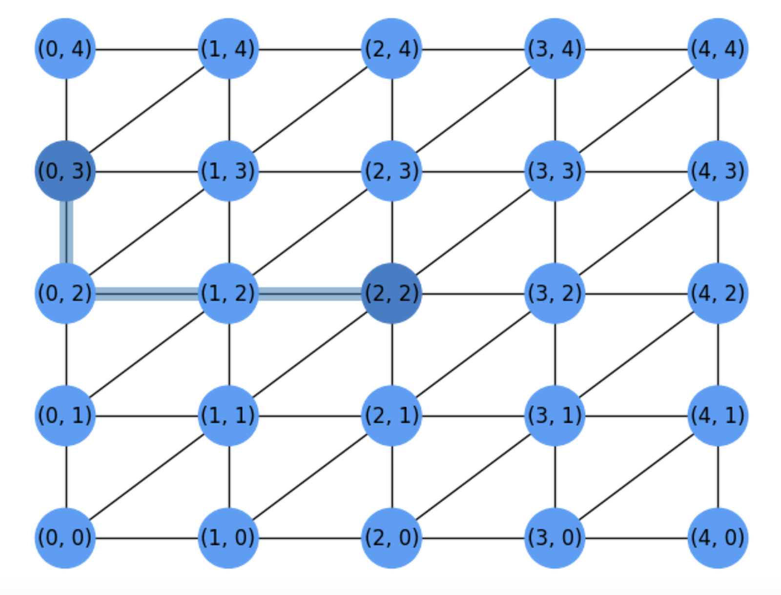
_images/Diagonal1.png — Fig. 5.1 \(6\)-neighborhood grid allowing right diagonals and SP.#

As we do not want to consider each particular case, it is better to systematize all the cases in a general algorithm. This is the so-called Dijkstra Algorithm after his author Edsger Dijkstra, who devised this method in 20 minutes.

5.1.1. Dijkstra Algorithm#

The Algorithm, described in pseudocode in Dijkstra can be summarized as follows.

Start at the source node \(s\) and visit its neighbors to find there the target \(t\) if possible. If this happens, the length of the SP is given by the edge \((s,t)\) and obviously it has length \(1\).
If the target \(t\) is not in the neigborhood of the source, we must close the source and continue the search from all its neighbors. In this case, the length of SP will be greater than \(1\).
Closing a node means that this node will be never visited later by the algorithm. We close a node once we select it as a candidate to belong to the SP. Closing node is implemented by removing it from a list of candidates \(L\).
In the beginning, all the nodes are included in \(L\). This is done in the initialization phase of the algorithm (steps 1 and 2).
Once a node is closed, we visit its neighbors still in \(L\) and check whether we can reach the target from them. This consists in updating their distance wrt the source. The nodes with shortest distances wrt the source have more chance to be selected for closing and verifying if they are the target.
The algorithm proceeds until there are no more candidates to visit (\(L\) is empty) or we have reached the target (step 3.2).

Algorithm 5.1 (Dijkstra)

Inputs Given a Network \(G=(V,E)\), a source node \(s\), and a target node \(t\)

Output Compute a path \(\Gamma\) from \(s\) to \(t\) of minimun length

for each node \(v\in V\):
1. dist[\(v\)]\(\;\leftarrow \infty\)
2. prev[\(v\)]\( \;\leftarrow -1\)
3. add \(v\) to \(L\)
dist[\(s\)]\(\;\leftarrow 0\)
while \(L\neq\emptyset\;\):
1. \(u\; \leftarrow\arg\min\) dist[\(u\)]\(\;, u\in L\)
2. if \(u = t\):
  1. break
3. remove \(u\) from \(L\)
4. for \(v\in\) neighbors(\(u\)):
  1. if \(v\in L\):
    1. new_dist\(\;\leftarrow\) dist[\(u\)] + \(w(u,v)\)
    2. if new_dist < dist[\(v\)]:
      1. dist[\(v\)]\(\;\leftarrow\) new_dist
      2. prev[\(v\)]\(\;\leftarrow u\)
return dist, prev

Source: Wikipedia

Let us show how to obtain the SP in Fig. 5.1.

Iteration 1

First of all, we visit the neighbors of the source \(s\) (we assume hat \(s\neq t\)). Visiting the neighbors of a node means expanding it.
To force such a expansion we have set \(dist[s]=0\). Since \(dist[v]=\infty\) for \(v\neq s\), this will force to select \(s\) at 3.1.
Then \(s\) is removed from \(L\) (step 3.3) because it is different from \(t\) and we proceed to visit its neighbors \(v\) (of \(u\)) which have not been expanded yet (still in \(L\)). See Fig. 5.2 the 6 neighbors of \(s=(2,2)\). They are explored sequentially (only the ones still belonging to \(L\)) in the for loop in 4.1.
In the above figure, we put oriented edges to show who is the expanded node (origin of the edge) and who are its neighbors (destinations of the edges). This means that the SP search can be traced by a search tree!

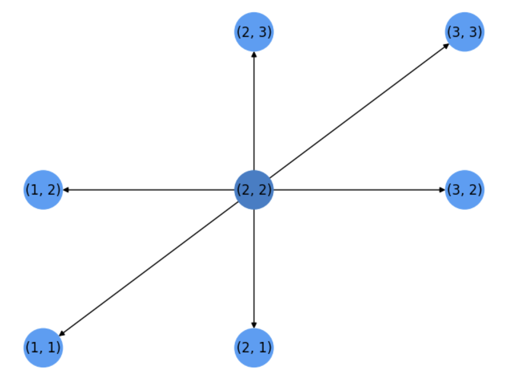
_images/DijkStep1.png — Fig. 5.2 Step 1. Expansion of source node.#

Therefore, for each neighbor \(v\) of the last expanded node \(u=(2,2)\) we try to update the distance of \(v\) wrt \(u\). Such a distance is encoded by \(w(u,v)\) which in principle is \(1\) unless we have positive edge weights.
The updated distances are stored in \(dist[\;]\) (where we had \(dist[s]=0\) and \(dist[v]=\infty\) for \(v\neq s\)) so that we can choose the next candidate node to expand which at this moment can be only a neighbor of \(u\). In general it can be any visited node (a neighbor of a expanded node) with the smallest distance wrt the source! (the may be many of them).
If a visited node becomes a candidate to expand we put in \(prev[\;]\) the latest node pointing to it. In this case, all the neighbors of \(s\) are candidates and they are pointed by \(s\). The only node not pointed by anyone is \(s\) itself, and this is why \(prev[s]=-1\) stays forever.

Iteration 2

At the end of the first iteration, all the neighbors \(v\) of \(u\) satisfy \(dist[v]=1\) and thus they are equally elegible to be expanded.
This is a remarkable feature of Dijkstra: the algorithm has no idea of what of the candidates is closer to the target. It only knows how far they are from \(s\). Dijkstra is blind to the target.
See Fig. 5.3. Casually, the algorithm chooses \((1,1)\) instead of other candidates farther from the target \(t=(0,3)\).

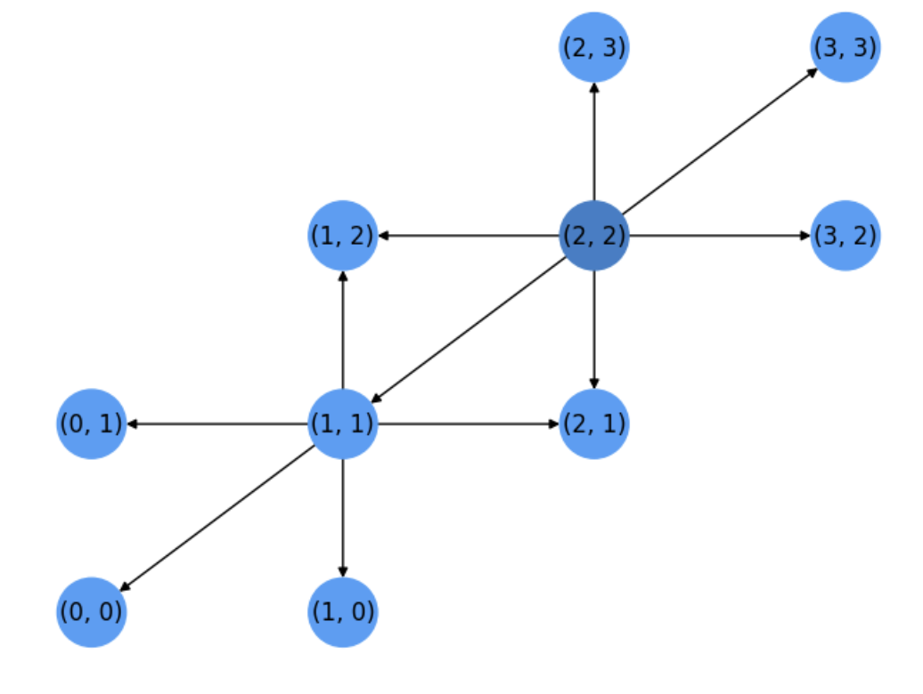
_images/DijkStep2.png — Fig. 5.3 Step 2. Expansion of node \((1,1)\).#

Note that some of the neighbors of the latest expanded node \(u=(1,1)\), namely \((2,1)\) and \((1,2)\), have been yet visited by the previous expanded node \(s=(2,2)\). As a result, their entries in \(dist[\;]\) are not \(\infty\) and their distances wrt the source will not change for the moment.
Only the distances wrt to the source of \((0,1)\), \((0,0)\) and \((1,0)\) will drop from \(\infty\) to \(2\). Thus, none of these nodes are candidates to be expanded. Only the common neighbors of \((2,2)\) and \((1,1)\) since they have \(dist[\;]=1<2\).
In particular, node \((1,2)\) will be chosen for expansion in the next iteration.

Iteration 3

See Fig. 5.4. Node \(u_3=(1,2)\) is expanded and some of its neighbors, \((2,3)\) and \((0,1)\) are common to the previous expanded nodes \(u_1=s=(2,2)\) and \(u_2=(1,1)\).
Dijkstra will expand any non expanded node of the source \(s=(2,2)\) before considering others since they are closer to it!
Actually, the next expanded node is \(u_4=(2,1)\)

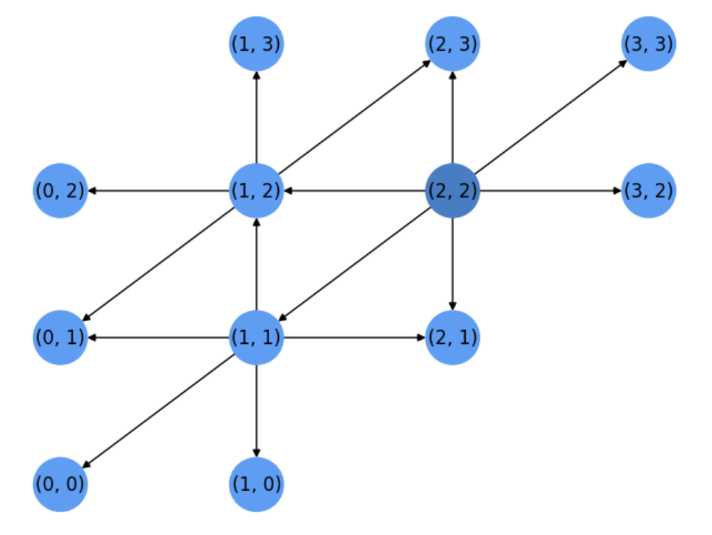
_images/DijkStep3.png — Fig. 5.4 Step 3. Expansion of node \((1,2)\).#

Iteration 4, and beyond

After expanding \(u_4=(2,1)\) it is the turn of \(u_5=(2,3)\) and then \(u_6=(3,2)\). See Fig. 5.5

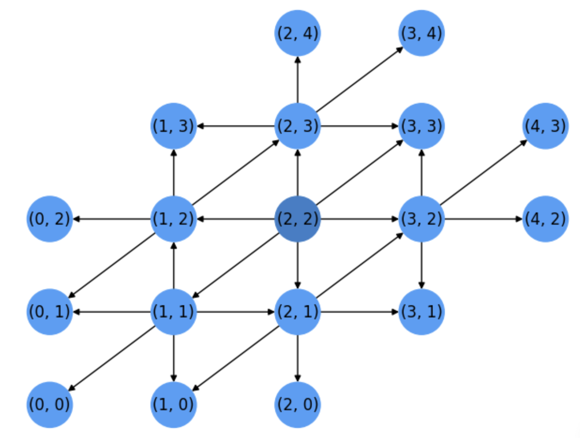
_images/DijkStep4-6.png — Fig. 5.5 Steps 4-6. Expansion of nodes \(u_4=(2,1), u_5=(2,3), u_6=(3,2)\).#

At this point, all the neighbors of the source \(s=(2,2)\) but \(u_7=(3,3)\) have been expanded and after expanding it we will consider nodes far away from the source in more than \(1\) unit.
Next nodes to expand will be: \(u_8=(0,0)\), \(u_9=(0,1)\), \(u_{10}=(0,2)\), all at distance \(2\) wrt the source. However the target \(t=(0,3)\), which is a neighbor of \(u_{10}=(0,2)\) but at distance \(3\) from \(s\), will not be expanded until all nodes at distance \(2\) wrt \(s\) are expanded: \(u_{11}=(1,0)\), \(u_{12}=(1,3)\), \(u_{14}=(2,0)\), \(u_{15}=(2,4)\), \(u_{16}=(3,1)\), \(u_{17}=(3,4)\), \(u_{18}=(4,2)\), \(u_{19}=(4,3)\) and \(u_{20}=(4,4)\) (who is a dead-end wrt the target). See the state of the search after expanding \(u_{20}=(4,4)\) in Fig. 5.6:

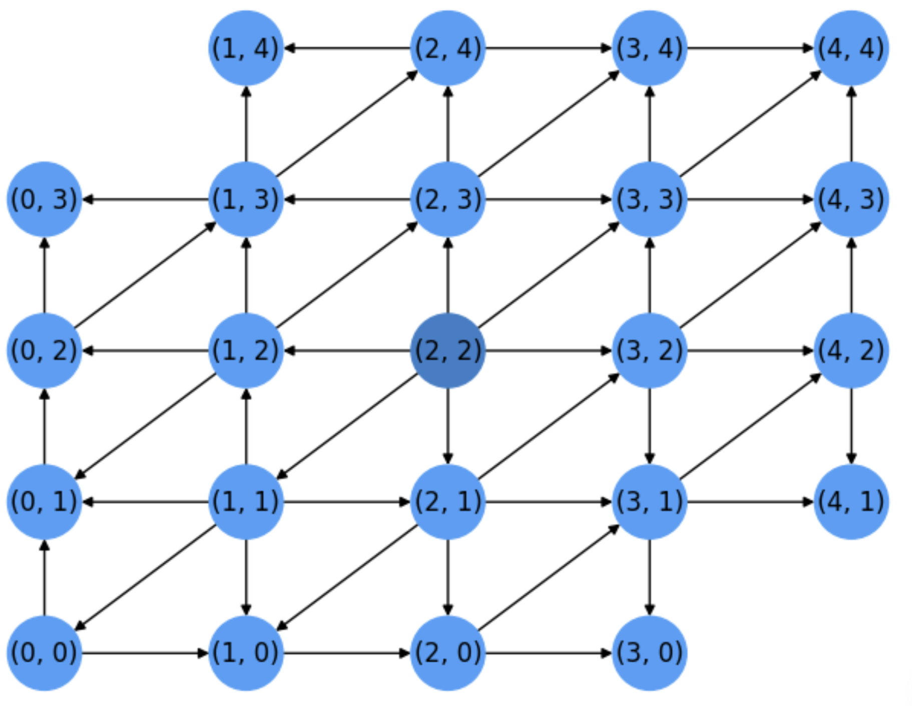
_images/DijkStep20.png — Fig. 5.6 Step 20. Right before expanding the target (which is yet visited long ago).#

Finally, \(u_{21}=(0,3)=t\) is the firts node at distance \(3\) from the source to be expanded. Actually \((1,4)\) or \((0,3)\) could be expanded before, but we were lucky and discovered the target in \(21\) steps!

Therefore, if the target is at distance \(d\) from the source it will be expanded by Dijkstra only when all the nodes at distance \(d-1\) from the source have been expanded yet. This is a Bread-First Search (BFS).

Exercise. In Fig. 5.7 we show a basic graph \(H\) with the shortest path between the source \(s=(0,0)\) and the target \(t=(2,3)\). Show: a) the number of iterations required by the Dijkstra algorithm as well as the search tree with a possible order of expansion of the nodes. b) What is the ratio between visited nodes and total nodes in \(H\)?.

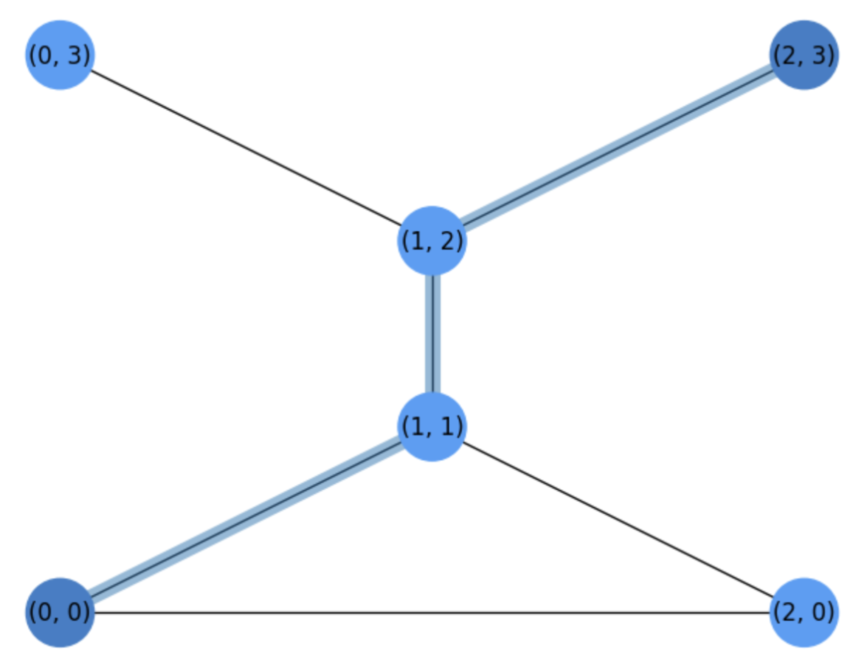
_images/ExerciseH.png — Fig. 5.7 Basic graph \(H\) for a Dijkstra Exercise.#

We commence by expanding the source \(u_1=s=(0,0)\) and then we visit its neigbors \((1,1)\) and \((2,0)\). Both have a distance \(1\) wrt to the source \(s\), so we select \(u_2=(2,0)\) for expansion. Next we select \(u_3=(1,1)\) (the other neighbor of the source at distance \(1\)). See the search tree in Fig. 5.8.

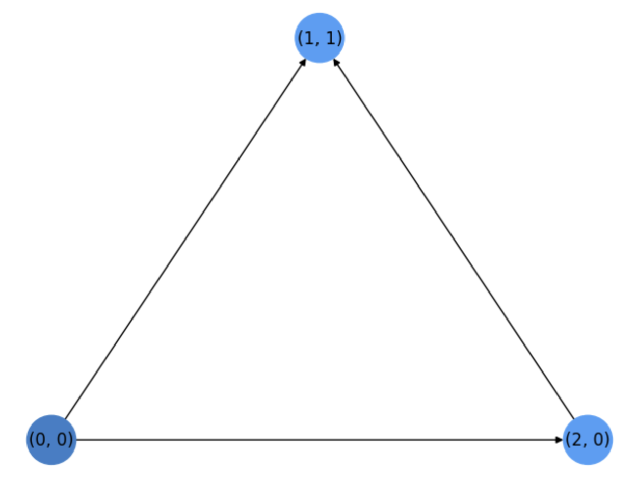
_images/ExerciseH2.png — Fig. 5.8 Search tree after two steps (before expanding \(u_3=(1,1)\))#

When expanding \(u_3=(1,1)\), only its neighbor \((1,2)\) has not been visited yet. In addition, since all the nodes at distance \(1\) wrt the source have been expanded, we expand \(u_4=(1,2)\) at distance \(2\) from the source and visit its neighbors \((0,2)\) and \((2,3)\). Since they are distance \(3\), one of them will be expanded once we verify that all nodes at distance \(2\) have been expanded, as it is the case.

Then we expand \(u_5=(0,3)\) which is a dead end wrt to the target and and finally the target \(u_6=t=(2,3)\). See the search tree before doing the last expansion in Fig. 5.9.

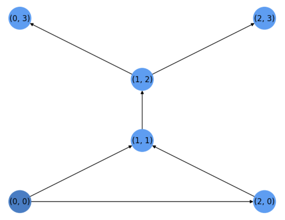
_images/ExerciseH3.png — Fig. 5.9 Search tree before expanding the target.#

Finally, as we have expanded all the nodes* in \(H\), the expansion ratio is \(1\).

Computational Complexity. How hard is to apply the Dijkstra algorithm wrt the number of nodes \(|V|\) and edges \(|E|\) in a graph \(G=(V,E)\)? To that end we use the Big-O notation (upper bound complexity) that you will study shortly.

The for loop for the distances initialization has complexity \(O(|V|)\).
How many steps can last the while loop? In the worst case, we iterate until the list \(L\) is empty. This means that all nodes have been expanded, which in principle means \(O(|V|)\) complexity. However, as many nodes have been expanded before a given one is expanded, we actually need to count the edges of the search tree. As a result, we may have \(O(|E|)\) complexity for sparse graphs and \(O(|E|=|V|^2)\) for dense ones.
Inside the while there are two main blocks: (a) computing the \(\arg\min\; dist[]\) and (b) expanding the node \(u\) and visit its neighbors \(v\).
- Computing the \(\arg\min\; dist[]\) is has a rough complexity of \(O(|V|)\).
- Running the for loop for visiting the u neighbors can be done in \(O(d_{max})\), where \(d_{max}\) is the maximun degree \(deg(v),v\in V\).
So, basically the complexity of the while loop is roughly \(O(|E|\cdot|V|)\).
However, as finding the \(\arg\min\; dist[]\) can be optimized for sparse graphs, we may have a worst-case complexity of \(\Theta((|E|+|V|)\log|V|)\) or even better \(\Theta(|E|+|V|\log|V|)\). Herein \(\Theta(.)\) means “on average”.
However, this almost quadratic complexity motivates also better algorithmic ways of going more straight to the target!

5.1.2. Heuristics and \(A^{\ast}\)#

AI algorithms often rely on a bit more sophisticated criteria for exanding a node:

Let \(g(u)\) an estimation of the shortest path distance wrt the source \(g^{\ast}(u)\). If the graph is not weighted, \(g^{\ast}(u)\) is the length of the shortest path from \(u\) to \(s\).
Now, we introduce \(h(u)\) as an estimation of \(h^{\ast}(u)\), namely the optimal (shortest) path distance wrt to the target \(t\). This function \(h(.)\) is called the heuristic.

Basically, \(g(u)\) estimates the work yet done, whereas \(h(u)\) estimates how promising is \(u\) to reach the target \(t\), i.e. the work to do. As a result, the so-called \(A^{\ast}\) algorithm consists of modifying the line 4.1.1 of Dijkstra (see AStar):

Algorithm 5.2 (\(A^{\ast}\) from Dijkstra)

for \(v\in\) neighbors(\(u\)):
1. if \(v\in L\):
  1. new_dist\(\;\leftarrow\) \(g(u)+ h(u)\)

where \(g(u)=\text{dist}[u] + w(u,v)\).

Therefore \(A^{\ast}\) can be seen as an extension of Dijkstra where the node selected for expansion minimizes

\[ f(u) = g(u) + h(u)\;. \]

Main idea. The underlying idea of \(A^{\ast}\) is that, Dijkstra uses only \(f(u) = g(u)\) but \(A^{\ast}\) is more informed than Dijkstra since it also includes \(h(u)\), i.e. \(f(u)= g(u)+ h(u)\) as a means of solving draws.

In other words, if several nodes \(u\) have the same value of \(g(u)\) and they are equally elegible for expansion by Dijkstra, \(A^{\ast}\) selects \(u = \arg\min g(u) + h(u)\).

Compare for instance Fig. 5.10 with Fig. 5.6. In both cases, we have \(s=(2,2)\) and \(t=(0,3)\). The \(A^{\ast}\) algorithm proceeds as follows:

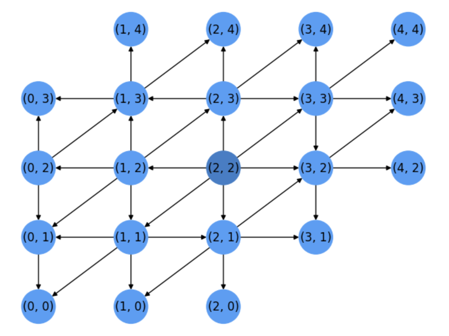
_images/AStarExample.png — Fig. 5.10 Search tree for \(A^{\ast}\).#

Expand \(u_1=s=(2,2)\) and visit all its neighbors.
Expand \(u_2=(1,2)\) since it is the neighbor of \(u_1\) closer to the target \(t\).
Expand \(u_3=(2,3)\), also a neighbor of \(u_1\). The node \((1,3)\) is not expanded before, despite it is closer to the target \(t\) because it has not been visited yet (it is not a neighbor of \(u_1\)).
Similarly, the remaining not-yet-expanded neighbors of \(u_1\) are expanded as follows: \(u_4=(1,1)\), \(u_5=(2,1)\), \(u_6=(3,3)\) and \(u_7=(3,2)\).
Next, it is the time to expand the nodes at distance \(2\) from the source \(s\), prioritizing those closer to the target \(t\). This results in expanding \(u_8=(0,2)\), \(u_9=(1,3)\) and \(u_{10}=(0,1)\).
Finally, from them we reach \(u_{11}=t=(0,3)\), i.e. the target if half iterations than Dijkstra!

How the heuristic is really chosen? In 2D grids, where each node \(u\) is anchored to a given Euclidean position \(P_u = (x_u,y_u)\), the heuristic function \(h(.)\) is chosen according to a given distance. The most obvious one is the Euclidean or air distance between \(P_u\) and \(P_t\) (the respective anchorings of \(u\) and the target \(t\)):

\[ h_E(u) = \sqrt{|x_u-x_t|^2 + |y_u-y_t|^2}\;. \]

Admissibility. Not all distances are compatible with every type of graph. Such a compatibility depends on how the optimal/perfect heuristic is computed. For a grid graph with right diagonals, as the one explored above, the true shortest-path distance \(h^{\ast}(s)\) between \(s=(2,2)\) and \(t=(0,3)\) is \(3\). One may argue that we do not know it in advance, and this is true. Actually, we do not need to know it. We only need to satisfy:

\[ h(u)\le h^{\ast}(u)\; \forall u\;, \]

so that the \(A^{\ast}\) algorithm guarantees that we find the optimal/shortest path. This property of an heuristic function is called admissibility and it is ensured by the above minoration, since it bassically says that we never over-estimate the distance to the target. Otherwise we could discard an optimal path.

Checking admissibility. Using the Pythagorean theorem we can easily show that \(h(u)\le h^{\ast}(u)\; \forall u\;.\) Actually, the Euclidean distance between \(s=(2,2)\) and \(t=(0,3)\) is \(\sqrt{|0-2|^2 + |2-3|^2}=\sqrt{5}<3\).You can check that such a distance is also valid for any pair of nodes.

However, consider the Manhattan Distance

\[ h_M(u) = |x_u-x_t| + |y_u-y_t|\;, \]

for grids with right diagonals. Such a distance is even better informed than the Euclidean distance since it satisfies \(h_E(s)\le h_M(s)\le h^{\ast}(s)\) for \(s=(2,2)\) and \(t=(0,3)\), but for \(t=(4,4)\) we have that \(h_M(s)=4>h^{\ast}(s)=2\). Therefore, \(h_M(.)\) is not-admissible for this kind of graphs, although:

The Manhattan distance it is the optimal choice \(h_M(u)=h^{\ast}(u)\) for \(4-\)neighborhood graphs.
The Euclidean distance is the optimal choice \(h_E(u)=h^{\ast}(u)\) for \(8-\)neighborhood graphs (including both right and left diagonals).

The Manhattan distance is a good example of Taxicab Geometry: if we move in a real city, basically we put the nodes at the crossroads and we cannot go through the building blocks. In other words, we ignore the Euclidean geometry which indeed has many benefits in many applications of AI.

5.2. Maximum Flow#

5.2.1. Bottlenecks, flows and capacities#

An essential characterization of a graph is to detect whether it has a bottleneck and where it is if any.

Considering herein only directed graphs or digraphs \(G(V,E)\), a bottleneck \(B\subseteq E\) is a subset \(B\) of the edges \(E\) where the information flow collapses.

See, for instance, Fig. 5.11 where we have a directed graph with two special nodes \(s=0\) (source) and \(t=5\) (target). In this section, source nodes can only send information (to their successors) whereas target nodes (or sinks) can only receive information(from their predecessors).

Each edge \(e=(u,v)\in E\) is labeled with a capacity \(c(u,v)\) which determines the amount of information that can be send through the edge. In this example the source \(s=0\) can send at most \(10\), say bits of information. Such an amount is called edge flow \(f(u,v)\) and it satisfies:

Bounded by capacity. Obviously, the flow along an edge is upper bounded by the edge’s capacity:

\[ \forall (u,v)\in E\;: f(u,v)\le c(u,v)\;. \]

Skew symmetry. During flow propagation, the flow from \(u\) to \(v\) is the opposite of the flow from \(v\) to \(u\):

\[ \forall (u,v)\in E\;: f(u,v) - f(v,u)\;. \]

Flow conservation. The total flow to a node is zero, except for \(s\) that produces flow, and \(t\) that consumes flow:

\[ \forall u\in V\;:u\neq s, u\neq t\Rightarrow \sum_{w\in V}f(u,w) = 0\;, \]

For instance, consider \(e=(2,4)\) in Fig. 5.11. Since the capacity of this edge is \(c(2,4)=25\), theoretically we could sent \(25\) units of flow from \(2\rightarrow 4\). However, this is impossible since:

Node \(2\) can only receive at most \(10\) units from the source and we must satisfy \(f(s,2)=f(2,4)\).
Node \(4\) can only receive at most \(16\) units of flow since \(f(4,1) + f(4,5)\le 16\).

Losless: The total flow leaving the source \(s\) must be equal to the the total flow reaching the sink \(t\):

\[ \sum_{(s,u)\in E} f(s,u) = \sum_{(v,t)\in E} f(v,t)\;. \]

In Fig. 5.11, if we send \(10\) units from \(s=0\) to \(1\) and another \(10\) units to \(2\), the sink \(t=5\) must end receiving \(20\) units. If, for instance, the capacity \(c(4,t)\) where \(5\), this could not be possible and it would imply that only \(15\) units can be produced at \(s\).

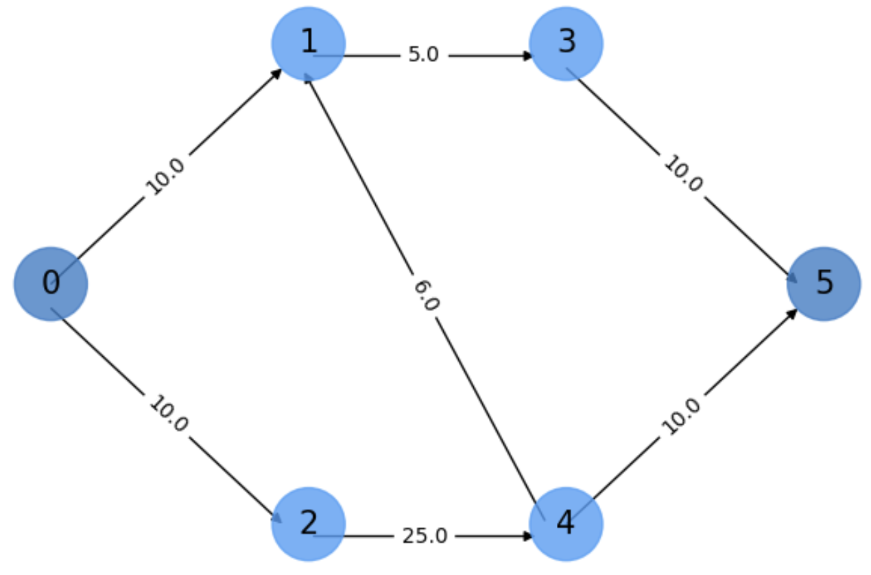
_images/SmallFlow.png — Fig. 5.11 Find a bottleneck in a directed graph.#

What is the bottleneck in the above figure? It seems obvious that the bottleneck is defined by the edges in \(G(V,E)\) with the smallest capacity, i.e. those that can constrain information transfer. Clearly, in our simple example the smallest capacity is \(c(1,3)=5\). Does it mean that we can only produce \(5\) units at \(s\)? Not really, this would happen if any of the paths from \(s\rightarrow t\) are forced to traverse \(e=(1,3)\). This is the case when the path \(\Gamma = s\rightarrow 2\rightarrow 4\rightarrow t\) doesn’t exist!

In other words, an edge or set of edges is really a bottleneck if it/them constrain the information flow between \(s\) and \(t\).

As a result, it seems reasonable to explore the paths between \(s\) and \(t\) and determine the weakest edges (those with smallest capacities) relative to each path.

5.2.2. The Ford-Fulkerson Method#

5.2.2.1. The general method#

A general approach to find the maximum flow between \(s\) and \(t\) in Fig. 5.11 could be as follows:

Find a path \(\Gamma_1\) between \(s\) and \(t\), for instance \(\Gamma_1 = s\rightarrow 1\rightarrow 3\rightarrow t\).
The weakest edge in \(\Gamma_1\) is the bottleneck of this path: \(e=(1,3)\) with \(c(1,3)=5\). This means that the maximum amount of information flowing through \(\Gamma_1\) will be \(f_1 = 5\).
Assign a flow equal to \(5\) to any edge in \(\Gamma_1\). Then we have

\[ f(s,1)=f(1,3)=f(3,t) = f_1 = 5\;. \]

Let us discover another path, say \(\Gamma_2 = s\rightarrow 2\rightarrow 4\rightarrow t\). The bottleneck of \(\Gamma_2\) is given by edges \((s,2)\) and \((4,5)\) with \(c(s,2)=c(4,5)=10\). As a result, although \(c(2,4)=25\) we can only send \(f_2=10\) units of flow through \(\Gamma_2\).
Assign a flow equal to \(10\) to any edge in \(\Gamma_2\). Then we have:

\[ f(s,2)=f(2,4)=f(4,t) = f_2 = 10\;. \]

At this point, the last path between \(s\) and \(t\), \(\Gamma_3 = s\rightarrow 2\rightarrow 4\rightarrow 1\rightarrow 3\rightarrow t\) is no longer explored. Why?

As the edge \((s,2)\) satisfies that \(c(s,2)=f(s,2)=f_2=10\) (we say that it is saturated) we are sure that any other path containing this edge will not return a better flow.
Although the edge \((s,1)\) is not saturated, (assume in this section to deal with directed graphs), path \(\Gamma_1\) contains a saturated edge \((1,3)\) with \(c(2,3)=f(s,1)=f_1=5\).

Then, the resulting total max-flow between \(s\) and \(t\) is \(f_1 + f_2 = 5 + 10 = 15\).

Therefore, this method, called the Ford-Fulkerson method (see Ford_Fulkerson) can be summarized as follows:

Set \(i=1\)
Find an augmenting path \(\Gamma_i\) and its bottleneck edge/s \(E_i\). This bottleneck provides the flow \(f_i\) and the corresponding saturated edges \(E_i\).
Update the flows of all the edges in \(\Gamma_i\).
Stop if no new augmenting paths can be found. Else,increment \(i = i+1\).
Return the total max-flow: \(F=\sum_i f_i\).

Algorithm 5.3 (Ford–Fulkerson)

Inputs Given a Network \(G=(V,E)\) with flow capacity \(c\), a source node \(s\), and a sink node \(t\)

Output Compute a flow \(f\) from \(s\) to \(t\) of maximum value

\(f(u, v) \leftarrow 0\) for all edges \((u,v)\)
while there is a path \(\Gamma\) from \(s\) to \(t\) in \(G_{f}\) such that \(c_{f}(u,v)>0\) for all edges \((u,v) \in \Gamma\):
1. Find \(c_{f}(\Gamma)= \min \{c_{f}(u,v):(u,v)\in \Gamma\}\)
2. for each edge \((u,v) \in \Gamma\)
  1. \(f(u,v) \leftarrow f(u,v) + c_{f}(\Gamma)\) (Send flow along the path)
  2. \(f(v,u) \leftarrow f(v,u) - c_{f}(\Gamma)\) (The flow might be “returned” later)
return \(f\).

5.2.2.2. Augmenting paths and Residual graph#

Some interesting elements in the above algorithm are as follows.

Augmenting paths. A central concept in this method are the \(s-t\) paths (directed paths between \(s\) and \(t\), \(\Gamma_i\)), proposed at each iteration. They are called augmenting paths because they do not contain any saturated edge.

Residual graph \(G_f=(V, E_f, c_f, f)\) is the graph where flows are updated. It works as follows:

\(E_f\) has \(2|E|\) edges, i.e. if \((u,v)\in E\) then we include both \((u,v)\) and \((v,u)\) in \(E_f\).
Initially all the edges \((u,v)\in E_f\) have \(f(u,v)=0\) (Step 1)
The residual capacity \(c(u,v)\in E_f\) is always given by

\[ c_f(u,v) = c(u,v) - f(u,v)\ge 0\;. \]

In the initial residual graph \(G_f\) (see Fig. 5.12) we have \(c_f(u,v)=c(u,v)\) for \((u,v)\in E\) and \(c_f(u,v)=0\) otherwise.

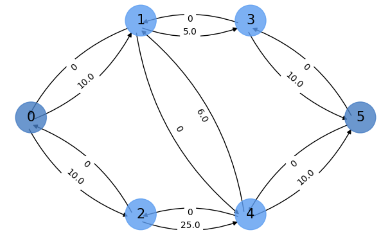
_images/SmallCapacities.png — Fig. 5.12 Initial residual graph.#

The residual graph is an auxiliary data structure to keeping track of the current capacity after each update the flows.
In addition, the residual graph registers the current flows, which always satisfy the above flow properties, in particular \(f(u,v)= - f(v,u)\) for \((u,v)\in E_f\).
Finally, it is very important to note that the all the edges in \(E_f\) can be used for finding augmenting paths, as we see below.

In Fig. 5.13, we show the final flows of \(G_f\) for the above example. Can you interpret the results?

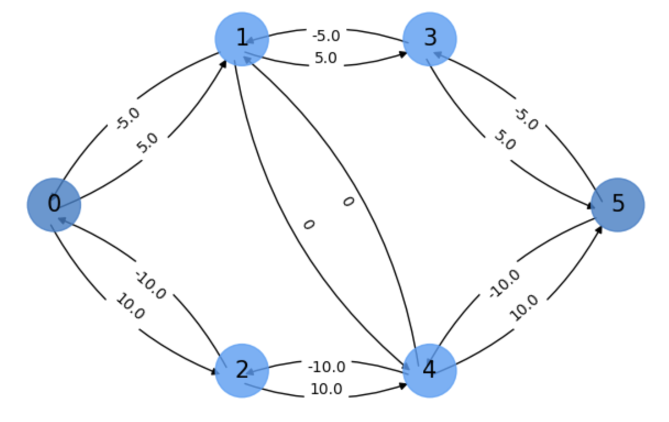
_images/SmallResult.png — Fig. 5.13 Final flows of the residual graph.#

We can see that the two augmented paths discoverd by the algorithm are

\[\begin{split} \begin{align} \Gamma_1 &= s\rightarrow 1\rightarrow 3\rightarrow t\\ \Gamma_2 &= s\rightarrow 2\rightarrow 4\rightarrow t\;.\\ \end{align} \end{split}\]

with respective flows \(f_1=5\) and \(f_2=10\). We know that from the above figure because:

The two leaving flows from \(s\) are respectively \(f_1=5\) and \(f_2=10\), exacly the same flows arriving to \(t\).
Edge \((4,1)\) is bypassed (it does not appear in any augmenting path) because both edges \((4,1)\) and \((1,4)\) have null flow!

How do we find the augmenting paths? As a result of the previous reasoning, all we need to solve the max-flow problem is to choose properly the augmenting paths \(\Gamma_i\). Actually, the algorithm for doing that is not specified in the Ford-Fulkerson method. Actually, we can send a random walker from \(s\) to \(t\) at each iteration. However, doing so may increase the complexity of the method.

Let us exemplify this by the following execution:

Use the \(G_f\) of Fig. 5.12.
Set all flows to zero \(f(u,v) = 0\;,\forall (u,v)\in E_f\).
Imagine, for instance, that the first augmenting path proposed by a random walker is

\[ \Gamma_1 = s\rightarrow 2\rightarrow 4\rightarrow 1\rightarrow 3\rightarrow t\;. \]

Looking at Fig. 5.11, the bottleneck of \(\Gamma_1\) is given by edge \((1,3)\) with \(c(1,3)=5\). As a result, all the edges in this path are assigned a flow \(f_1=5\). The edge \((s,2)\) is clearly unsaturated, and therefore it can be used in subsequent paths.

For instance, suppose that the second augmenting path proposed by a random walker is quite shorter (in terms of the number of edges) than \(\Gamma_1\):

\[ \Gamma_2 = s\rightarrow 1\rightarrow 4\rightarrow t\;. \]

Remember: we can do that because the all the edges in \(E_f\) can be used for finding augmenting paths!

The current flows of the edges in this path are:

\[\begin{split} \begin{align} f(s,1)&=0\;\text{with residual capacity}\; c_f(s,1)=10-0 = 10\\ f(1,4)&=-5\;\text{with residual capacity}\; c_f(1,4)=0-(-5) = 5\\ f(4,t)&=0\;\text{with residual capacity}\; c_f(4,t)=10-0 = 10\\ \end{align} \end{split}\]

and the respective negative values for the reverse edges. The current flows in the other edges are:

\[\begin{split} \begin{align} f(s,2)&=5\;\text{with residual capacity}\; c_f(s,2)=10-5 = 5\\ f(2,4)&=5\;\text{with residual capacity}\; c_f(2,4)=10-5 = 5\\ f(4,1)&=5\;\text{with residual capacity}\; c_f(4,1)=6-5 = 1\\ f(1,3)&=5\;\text{with residual capacity}\; c_f(1,3)=5-5 = 0\\ f(3,5)&=5\;\text{with residual capacity}\; c_f(3,5)=10-5 = 5\\ f(s,1)&=f(1,s)=0\;\text{with residual capacity}\; c_f=10-0 = 10\\ \end{align} \end{split}\]

respective negative values for the reverse edges.

Since the bottleneck of \(\Gamma_2=s\rightarrow 1\rightarrow 4\rightarrow t\) is given (according to Step 2.1) by

\[ f_2=\min(c_f(s,1), c_f(1,4), c_f(4,t)) = \min(10, 5, 10) = 5 \]

we will update the flows in the edges of \(\Gamma_2\) (Step 2.2) as follows:

\[\begin{split} \begin{align} f(s,1)&= 0 + 5 = 5\;\text{whereas the reverse flow becomes}\; f(1,s)=0-5 = -5\\ f(1,4)&=-5+ 5 = 0\;\text{whereas the reverse flow becomes}\; f(4,1)=5-5 = 0\\ f(4,t)&= 0 + 5 = 5\;\text{whereas the reverse flow becomes}\; f(t,4)=0-5 = -5\;.\\ \end{align} \end{split}\]

Herein, we have recovered the flow \(f(1,4)\) which increases from \(-5\) to \(0\). Therefore, edges \((1,4)\) and \((4,1)\) are still unsaturated since the capacity is \(6\).

Therefore: the fact that an edge appears with zero flow in the final result happens if it has been part of an augmeted path and then of another in the reverse direction which has restored the flow. This is actual the purpose of Step 2.2.

5.2.2.3. Sub-optimal traps#

After the second step, note that the total flow is \(f_1 + f_2 = 5 + 5 = 10\) which is not optimal at all (we know that the max-flow for this example is \(15\)).

Actually, this path \(\Gamma_2 = s\rightarrow 1\rightarrow 4\rightarrow t\) can be taken again. What does happen if \(\Gamma_3=\Gamma_2\)?

First of all, the flows and current residual capacities of the edges in this path are

\[\begin{split} \begin{align} f(s,1)&= 5\;\text{with residual capacity}\; c_f(s,1)=10-5 = 5\\ f(1,4)&= 0\;\text{with residual capacity}\; c_f(1,4)=6-0 = 6\\ f(4,t)&= 5\;\text{with residual capacity}\; c_f(4,t)=10-5 = 5\\ \end{align} \end{split}\]

Secondly, the bottleneck of this path is

\[ f_3 = \min(c_f(s,1),c_f(1,4),c_f(4,t)) = \min(5, 6, 5) = 5\;. \]

Then, the new flows for these edges are:

\[\begin{split} \begin{align} f(s,1)&= 5 + 5 = 10\;\text{whereas the reverse flow becomes}\; f(1,s)=-5-5 = -10\\ f(1,4)&= 0 + 5 = 5\;\text{whereas the reverse flow becomes}\; f(4,1)=0-5 = -5\\ f(4,t)&= 5 + 5 = 10\;\text{whereas the reverse flow becomes}\; f(t,4)=-5 -5 = -10\;.\\ \end{align} \end{split}\]

In this way, the total flow is \(f_1 + f_3 = 5 + 5 = 10\), still suboptimal. However, we have saturated both the edges \((s,1)\) and \((4,t)\) and this path \(\Gamma_3\) can not be used again.
Instead of that, we will discover the path

\[ \Gamma_{4} = s\rightarrow 2\rightarrow 4\rightarrow t\;, \]

which will provide the optimal max-flow: \(f_1 + f_4 = 5 + 10 = 15\).

In other words, if we have the bad luck of choosing a path whose edges are not saturated, but the maximum runing through these edges is, say \(f\), we can re-use this path until the flow of one of it edges reaches \(f\) and gets saturated.
As we can potential visit all edges of \(E_f\) (if the unsaturated path is very long), the complexity of this method is \(O(f\cdot|E|)\), that is, it depends on the value of the maximum flow running through the graph!
To fully understand this complexity we propose the following simple exercise.

Exercise. In Fig. 5.14 we show a basic digraph \(G\) with \(s=0\) and \(t=3\), illustrating the worst case for the Ford-Fulkerson method. It happens if we select alternatively the following paths

\( \begin{align} \Gamma_{odd} &= s\rightarrow 1\rightarrow 2\rightarrow t\\ \Gamma_{even} &= s\rightarrow 2\rightarrow 1\rightarrow t\\ \end{align} \)

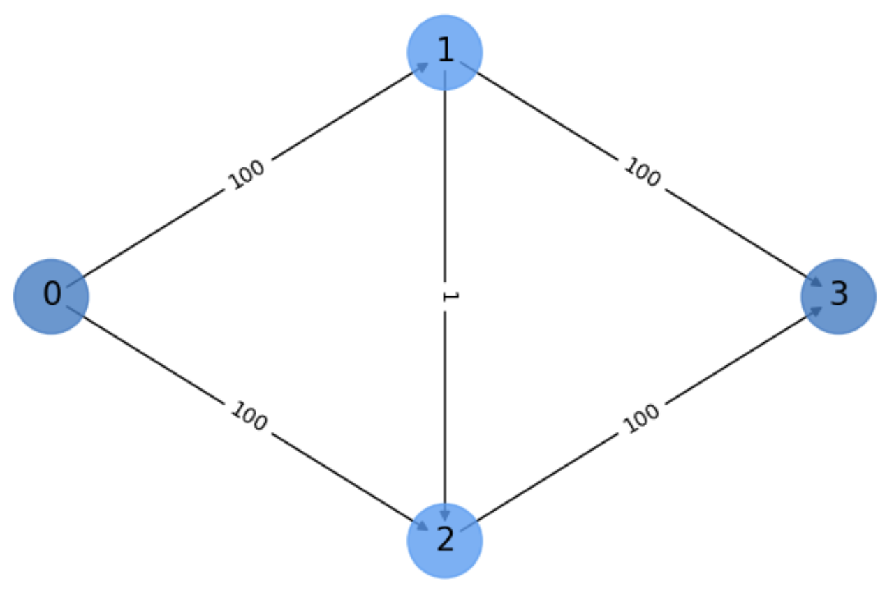
_images/SmallExercise.png — Fig. 5.14 Illustrating the worst case of Ford-Fulkerson.#

Remember that \(\Gamma_{even}\) can be selected because we search paths in the residual graph. The initial residual graph \(G_f\) is shown in Fig. 5.15

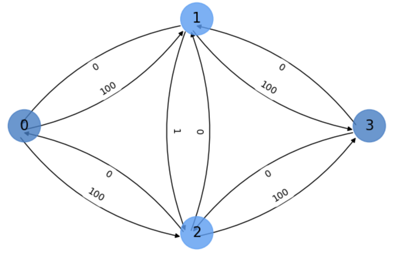
_images/SmallExerciseRes.png — Fig. 5.15 Initial residual graph \(G_f\) of the exercise.#

Why this is the worst case of the Ford-Fulkerson method?

Iteration 1: After setting all flows to \(0\), we select the path \(\Gamma_{odd} = s\rightarrow 1\rightarrow 2\rightarrow t\). Obviously, the bottleneck is given by \(c_f(1,2)=1\). The resulting flows of the edges in \(\Gamma_{odd}\) and their residual capacities are:

\( \begin{align} f(s,1)&= 0 + 1 = 1\;\text{with residual capacity}\; c_f(s,1)=100-1 = 99\\ f(1,s)&= 0 - 1 = -1\;\text{with residual capacity}\; c_f(1,s)=0-(-1) = 1\\ \mathbf{f(1,2)}&= 0 + 1 = 1\;\text{with residual capacity}\; \mathbf{c_f(1,2)=1-1 = 0}\\ f(2,1)&= 0 - 1 = -1\;\text{with residual capacity}\; c_f(2,1)=0-(-1) = 1\\ f(2,t)&= 0 + 1 = 1\;\text{with residual capacity}\; c_f(1,2)=100-1 = 99\\ f(t,2)&= 0 - 1 = -1\;\text{with residual capacity}\; c_f(t,2)=0-(-1) = 1\\ \end{align} \)

As a result, edge \((1,2)\) is saturated and we cannot use the path \(\Gamma_{even}\) for the moment.

Iteration 2: Let us use then \(\Gamma_{even} = s\rightarrow 2\rightarrow 1\rightarrow t\), because \(c_f(2,1)=1>0\). The bottleneck of this path is actually given by \(c_f(2,1)=1\). The resulting flows of the edges in \(\Gamma_{even}\) and their residual capacities are:

\( \begin{align} f(s,2)&= 0 + 1 = 1\;\text{with residual capacity}\; c_f(s,2)=100-1 = 99\\ f(2,s)&= 0 - 1 = -1\;\text{with residual capacity}\; c_f(2,s)=0-(-1) = 1\\ \mathbf{f(2,1)}&= -1 + 1 = 0\;\text{with residual capacity}\; \mathbf{c_f(2,1)=0- 0 = 0}\\ f(1,2)&= 1 - 1 = 0\;\text{with residual capacity}\; c_f(1,2)=1- 0 = 1\\ f(1,t)&= 0 + 1 = 1\;\text{with residual capacity}\; c_f(1,t)=100-1 = 99\\ f(t,1)&= 0 - 1 = -1\;\text{with residual capacity}\; c_f(t,1)=0-(-1) = 1\\ \end{align} \)

Iteration 3: We cannot use \(\Gamma_{even} = s\rightarrow 2\rightarrow 1\rightarrow t\), because \(c_f(2,1)=0\), but we can use again \(\Gamma_{odd} = s\rightarrow 1\rightarrow 2\rightarrow t\) since \(c_f(1,2)=1>0\). Doing so, we have again a bottlenec of \(1\) and:

\( \begin{align} f(s,1)&= 1 + 1 = 2\;\text{with residual capacity}\; c_f(s,1)=100-2 = 98\\ f(1,s)&= - 1 - 1 = -2\;\text{with residual capacity}\; c_f(1,s)=0-(-2) = 2\\ \mathbf{f(1,2)}&= 0 + 1 = 1\;\text{with residual capacity}\; \mathbf{c_f(1,2)=1-1 = 0}\\ f(2,1)&= 0 - 1 = -1\;\text{with residual capacity}\; c_f(2,1)=0-(-1) = 1\\ f(2,t)&= 1 + 1 = 2\;\text{with residual capacity}\; c_f(2,t)=100-2 = 98\\ f(t,2)&= -1 - 1 = -2\;\text{with residual capacity}\; c_f(t,2)=0-(-2) = 2\\ \end{align} \)

After three iterations, we have enough evidence to show that:

(a) Every time we run through \((1,2)\) we push an additional unit of flow through it, thus increasing the flow \(f(s,1)\), and as a result we saturate this edge \((1,2)\) and we enable the edge \((2,1)\).

(b) Then, if we choose to run through \((2,1)\), we increase the flow \(f(s,2)\) and as a result we saturate \((2,1)\) and we enable \((1,2)\)

Therefore, after \(2\cdot 100\) iterations, we are able to saturate both \(\Gamma_{odd}\) and \(\Gamma_{even}\), thus sending \(200\) units. Since each iteration takes almost all the edges in \(E\), the time complexity if of order \(O(f\cdot |E|)\).

The take to home message of the above exercise is to show that in the absence of a systematic (not random) way of choosing the paths, the Ford-Fulkerson method has a complexity which depends on the flow values. If our flows are as those in the example (we have a leaking link \((1,2)\) with a very small flow), this path choosing leads to the worst case of the method.

5.2.3. The Edmonds-Karp Method#

This method basically addresses exactly the point of incorporating a systematic way of exploring the augmenting paths. Basically, it consists in incorporating a BFS (Breadth-First-Search) method, such as the Dijkstra algorithm, in the Step 2 of the Ford-Fulkerson method (see Edmonds_Karp).

Algorithm 5.4 (Edmonds-Karp)

Inputs Given a Network \(G=(V,E)\) with flow capacity \(c\), a source node \(s\), and a sink node \(t\)

Output Compute a flow \(f\) from \(s\) to \(t\) of maximum value

\(f(u, v) \leftarrow 0\) for all edges \((u,v)\)
while there is a BFS shortest path \(\Gamma\) from \(s\) to \(t\) in \(G_{f}\) such that \(c_{f}(u,v)>0\) for all edges \((u,v) \in \Gamma\):
1. Find \(c_{f}(\Gamma)= \min \{c_{f}(u,v):(u,v)\in \Gamma\}\)
2. for each edge \((u,v) \in \Gamma\)
  1. \(f(u,v) \leftarrow f(u,v) + c_{f}(\Gamma)\) (Send flow along the path)
  2. \(f(v,u) \leftarrow f(v,u) - c_{f}(\Gamma)\) (The flow might be “returned” later)
return \(f\).

Some precisions have to be made at this point:

The BFS looks for the shortest paths (in terms of the number of edges) between \(s\) and \(t\) in the residual graph.
Shortest paths are more interesting than random walkers or even DFS (Depth-First Search) because the longer the path the more probable is to find a leaking edge (an edge with a very small capacity wrt to others) in it. Long paths usually result in the worst case of the algorithm.

Actually, the worst case of Ford-Fulkerson illustrated in Fig. 5.15, is easily avoided by finding the two paths:

\[ \Gamma_1 = s\rightarrow 1\rightarrow t \]

and

\[ \Gamma_2 = s\rightarrow 2\rightarrow t \]

thus avoiding the bottleneck edge \((1,2)\) (see Fig. 5.16, where the total flow is \(100 + 100 = 200\)).

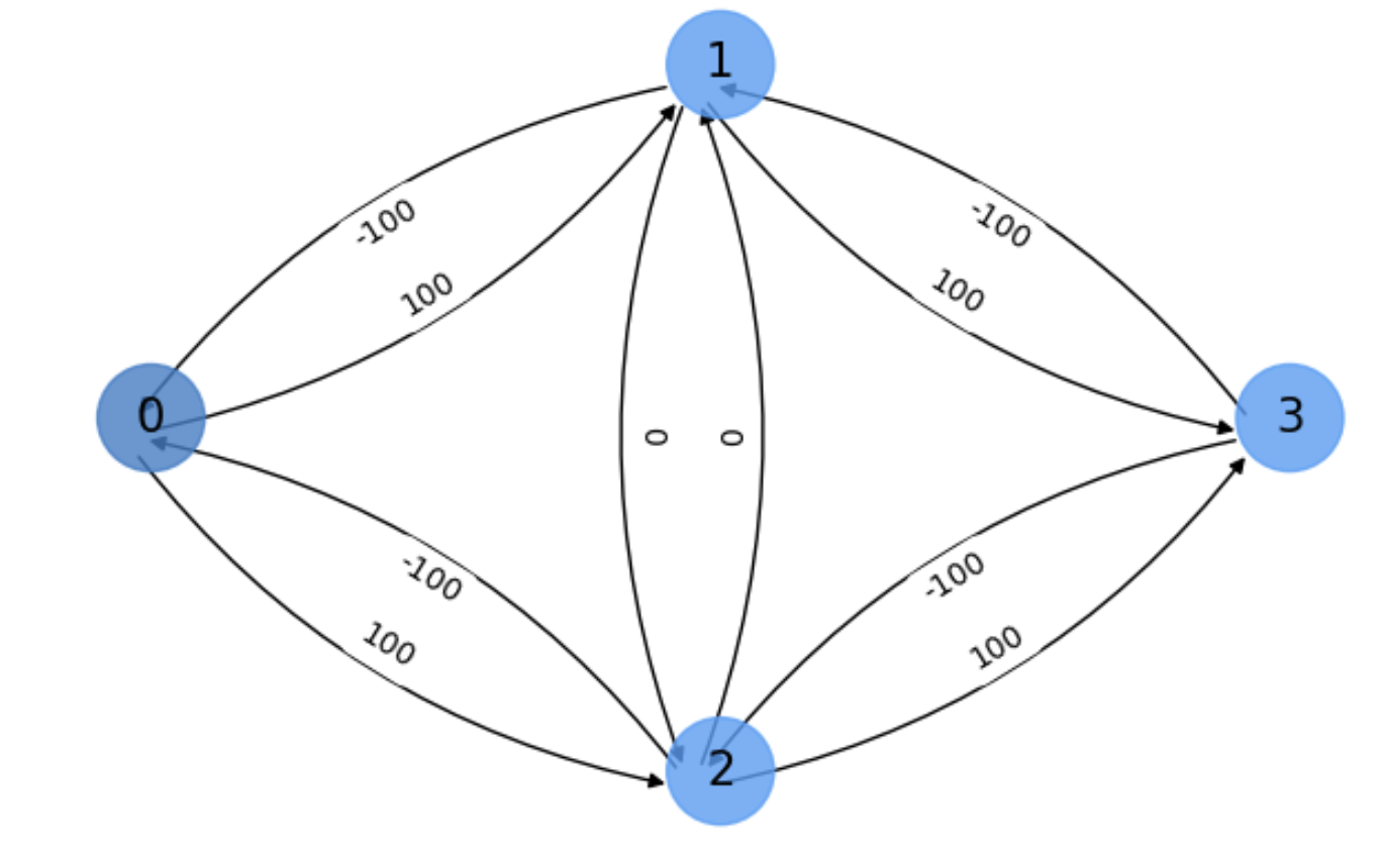
_images/SmallExerciseResFinal.png — Fig. 5.16 Final residual graph \(G_f\) of the exercise.#

Therefore: the fact that an edge appears with zero flow in the final result also happens when we avoid this edge (remember that the flow is set to \(0\) initially for all edges). .

Complexity. Concerning the complexity of Edmonds-Karp (E-K), since each iteration requires to run a BFS algorithm such as Dijkstra, with complexity \(O(|V|\cdot|E|)\) one may expect this complexity for E-K. However:

On each iteration of the algorithm, the shortest path between the source and all other vertices in the residual graph must increase monotonic. That is, it is always either non-decreasing or increasing. As a result, the path in the real graph is decreasing. This bounds the length of one iteration of Edmonds-Karp to \(O(|E|)\).
No modification to the residual graph ever reduces the distance from the source to any vertex; with this, and the fact that BFS always finds a shortest path, it’s possible to show that after finding at most \(|V|\cdot |E|\) augmenting paths, no source-to-sink path remains in the residual graph.
Then, the total complexity is \(O(|V|\cdot |E|^2)\).

Exercise. In Fig. 5.17 we show a digraph \(G\) with \(s=0\) and \(t=10\), illustrating the general case for the E-K method. Assume that you are given the augmenting paths discovered by the BFS algorithm. In this case we have used the bidirectional BFS exploited by Networkx. We have, ayway, the paths:

\( \begin{align} \Gamma_{1} &= s\rightarrow 1\rightarrow 4\rightarrow 7\rightarrow t\\ \Gamma_{2} &= s\rightarrow 2\rightarrow 5\rightarrow 8\rightarrow t\\ \Gamma_{3} &= s\rightarrow 3\rightarrow 6\rightarrow 8\rightarrow t\\ \end{align} \)

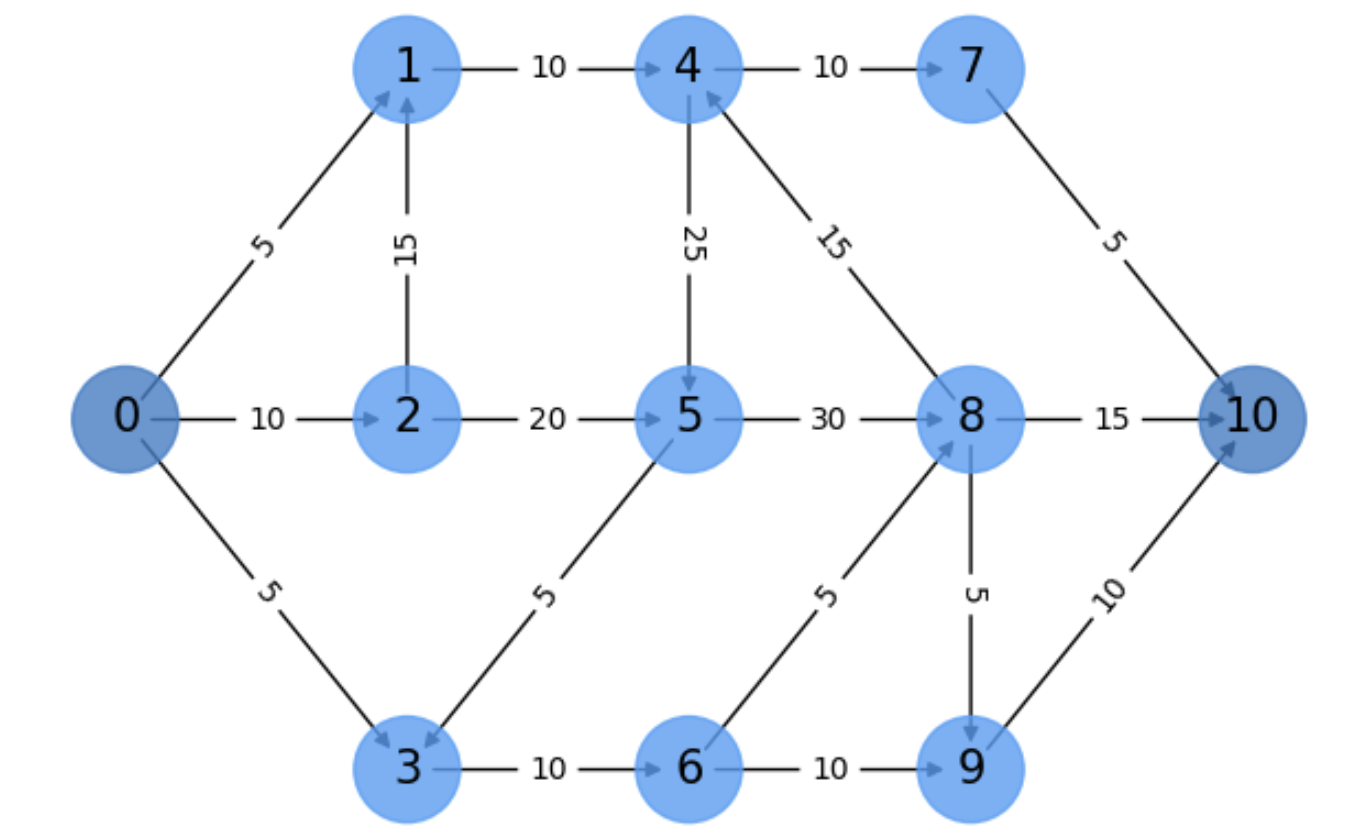
_images/BigExercise.png — Fig. 5.17 A more complex E-K example.#

The exercise consists in explaining how these paths contribute to find the maximal flow and what is it

Iteration 1. After initializing all the flows in the residual graph as \(f=0\), let us start by \( \Gamma_{1} = s\rightarrow 1\rightarrow 4\rightarrow 7\rightarrow t\). Its bottleneck is at edge \(e=(s,1)\) (or at \(e=(7,t)\)) where we have \(c(e)=5\). Anyway, this leads to the following flows and residual capacities:

\( \begin{align} \mathbf{f(s,1)}&= 0 + 5 = 5\;\text{with residual capacity}\; \mathbf{c_f(s,1)}=5-5 = 0\\ f(1,s)&= 0 - 5 = -5\;\text{with residual capacity}\; c_f(1,s)=0-(-5) = 5\\ f(1,4)&= 0 + 5 = 5\;\text{with residual capacity}\; c_f(1,2)=10-5 = 5\\ f(4,1)&= 0 - 5 = -5\;\text{with residual capacity}\; c_f(2,1)=0-(-5) = 5\\ f(4,7)&= 0 + 5 = 5\;\text{with residual capacity}\; c_f(4,7)=10-5 = 5\\ f(7,4)&= 0 - 5 = -5\;\text{with residual capacity}\; c_f(4,7)=0-(-5) = 5\\ \mathbf{f(7,t)}&= 0 + 5 = 5\;\text{with residual capacity}\; \mathbf{c_f(7,10)}=5-5 = 0\\ f(t,7)&= 0 - 5 = -5\;\text{with residual capacity}\; c_f(t,7)=0-(-5) = 5\\ \end{align} \)

This results in the saturation of the bottleneck edges \((s,1)\) and \((7,t)\). These two edges cannot be used in other augmenting paths. The length of \(\Gamma_1\) in terms of number of edges is \(|\Gamma_1|=4\).

Iteration 2. As we cannot take a path with the saturated edge \((t,1)\) the algorithm picks another shortest path in the residual graph. In this case, it takes \(\Gamma_{2} = s\rightarrow 2\rightarrow 5\rightarrow 8\rightarrow t\) also with length \(|\Gamma_2|=4\) as it has \(\Gamma_1\). The bottleneck is given by the edge \(e=(t,2)\) with capacity \(c(t,2)=10\). Next, we proceed to update flows and residual capacities:

\( \begin{align} \mathbf{f(s,2)}&= 0 + 10 = 10\;\text{with residual capacity}\; \mathbf{c_f(s,2)}=10-10 = 0\\ f(2,s)&= 0 - 10 = -10\;\text{with residual capacity}\; c_f(2,s)=0-(-10) = 10\\ f(2,5)&= 0 + 10 = 10\;\text{with residual capacity}\; c_f(1,2)=20-5 = 10\\ f(5,2)&= 0 - 10 = -10\;\text{with residual capacity}\; c_f(5,2)=0-(-10) = 10\\ f(5,8)&= 0 + 10 = 10\;\text{with residual capacity}\; c_f(5,8)=30-10 = 20\\ f(8,5)&= 0 - 10 = -10\;\text{with residual capacity}\; c_f(8,5)=0-(-10) = 10\\ f(8,t)&= 0 + 10 = 10\;\text{with residual capacity}\; \mathbf{c_f(8,10)}=15-10 = 5\\ f(t,8)&= 0 - 10 = -10\;\text{with residual capacity}\; c_f(t,8)=0-(-10) = 10\\ \end{align} \)

This results in the saturation of edge \((t,1)\) and thus we cannot use it in any other paths. At this point, note that each augmenting path discarts many others in the future and this is why this motivates the computational complexity described above.

Iteration 3. The remaining augmenting paths cannot use neither the edge \((s,1)\) not the edge \((s,2)\). As a result, they must depart from \((s,3)\). Some of them have length \(4\) (please identify them) but the algorithm chooses \(\Gamma_{3} = s\rightarrow 3\rightarrow 6\rightarrow 8\rightarrow t\) also with length \(|\Gamma_3|=4\). Its bottleneck is the edges \(e=(t,3)\) and \(e=(6,8)\) with capacities \(c(e)=5\). This results in the following flows and residual capacities.

\( \begin{align} \mathbf{f(s,3)}&= 0 + 5 = 5\;\text{with residual capacity}\; \mathbf{c_f(s,3)}=5-5 = 0\\ f(3,s)&= 0 - 5 = -5\;\text{with residual capacity}\; c_f(s,s)=0-(-5) = 5\\ f(3,6)&= 0 + 5 = 5\;\text{with residual capacity}\; c_f(3,6)=10-5 = 5\\ f(6,3)&= 0 - 5 = -5\;\text{with residual capacity}\; c_f(6,3)=0-(-5) = 5\\ \mathbf{f(6,8)}&= 0 + 5 = 5\;\text{with residual capacity}\; \mathbf{c_f(6,8)}=5-5 = 0\\ f(8,6)&= 0 - 5 = -5\;\text{with residual capacity}\; c_f(8,6)=0-(-5) = 5\\ f(8,t)&= 10 + 5 = 15\;\text{with residual capacity}\; \mathbf{c_f(8,t)}=10-5 = 5\\ f(t,8)&= -10 - 5 = -15\;\text{with residual capacity}\; c_f(t,8)=0-(-15) = 15\\ \end{align} \)

Total flow. Since we have \(f_1 = 5\), \(f_2 = 10\), and \(f_3 = 5\), the total flow is \(f_1 + f_2 + f_3 = 20\).

5.3. Cycles: Hamiltonian and Eulerian#

Cycles (circuits) in graphs are very interesting for AIers since they are linked with intriguing combinatorial problems, some of them being NP-Hard. In this regard, it seems convenient to explore one of these problems, namely The Travelling Salesman Problem (TSP) where the study of two main types of cycles Hamiltonian Cycles and Eulerian Cycles play a key role.

5.3.1. The Travelling Salesman Problem#

A travelling salesman optimizes its visits as follows: He/She has to visit \(n\) cities \(c_1, c_2,\ldots, c_n\) once in such a way that after visiting the last city the traveller comes back to the departing one (i.e. we have a cycle). This type of cycle is called a Hamiltonial cycle.

In the metric version of the problem, each city has associated a location on the plane \((x_i, y_i)\), meaning that we may exploit the Euclidean distances between cities to decide the optimal strategy. Actually the algorithm must find the minimum cost cycle. A bit more formally, we must find a permutation \(\pi(1,\ldots,n)\) of the cities so that

\[ \pi = \arg\min d(\pi(1),\pi(2)) + d(\pi(2),\pi(3)) + \ldots + d(\pi(n-1),\pi(n)) + d(\pi(n),\pi(1))\;. \]

where \(d(\pi(i),\pi(j))=\sqrt{(x_{\pi(i)} - x_{\pi(j)})^2 + (y_{\pi(i)} - y_{\pi(j)})^2}\). Since we have \(n!\) permutations of \(n\) cities, the fact of looking for a specific permutation, the one leading to the minimum cost, makes the problem NP-Hard. All we can do is to propose reasonable polynomial approximations.

In the following, we are going to specify the steps of the Christophides algorithm (see Christophides), which is the approximation used in Networkx.

Algorithm 5.5 (Christophides)

Inputs Given a complete graph \(G=(V,E,w)\) with edge weights (distances) \(w:E\rightarrow\mathbb{R}\),i.e. \(w(i,j)=d(i,j)\).

Output Return a Hamiltonian cycle \(\Gamma\).

Find a Minimum Spanning Tree \(T\).
Let \(O\) be the set of nodes with odd degree in \(T\). Find a minimum-cost perfect matching \(M\).
Add the set of edges of \(M\) to \(T\).
Find an Eulerian Tour \(\Gamma^0\).
Shortcut \(\Gamma^0\) to make a Hamiltonian Cycle \(\Gamma\).
return \(\Gamma\).

This algorithm is the one used for approximating the TSP in Fig. 5.18, where the route of the traveller is:

\[ \Gamma = 0\rightarrow 6\rightarrow 1\rightarrow 4\rightarrow 8\rightarrow 3\rightarrow 5\rightarrow 7\rightarrow 2\rightarrow 9\rightarrow 0\;. \]

For the sake of simplicity, we only show in the figure the closest edges to each of the \(|V|=10\) nodes in \(G\).

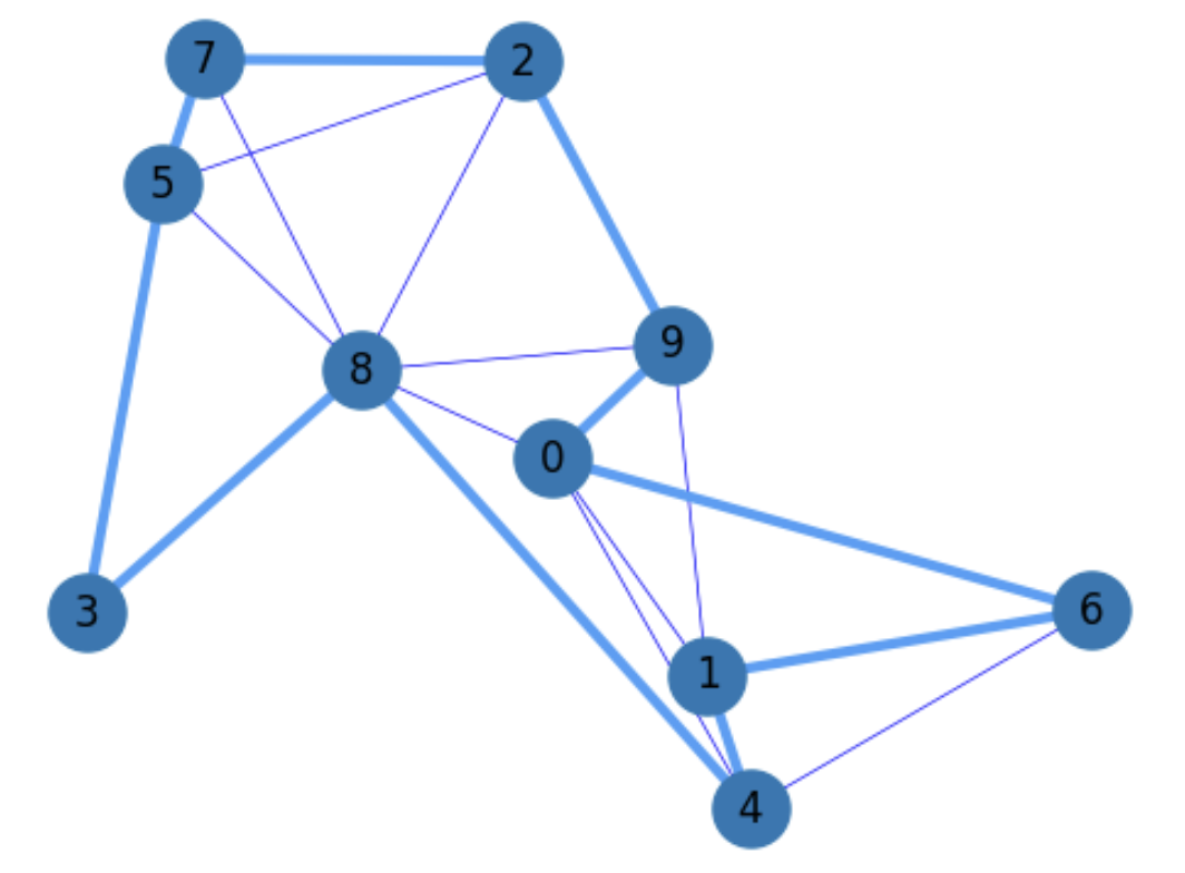
_images/TSP1.png — Fig. 5.18 Complete graph and a TSP solution (in bold).#

5.3.1.1. Minimum Spaning Trees#

The first step for the above TSP algorithm consists in computing a Minimum Spanning Tree (MST).

First of all, a tree is nothing but a graph without cycles. Given the nodes \(V\) of \(G=(V,E,w)\), we must find a subgraph \(T=(V,E',w)\), with \(E'\subseteq E\), satisfying:

\(T\) is a connected graph, i.e. it links all the nodes in \(V\).
\(T\) is a tree i.e. it does not have cycles/circuits.
The sum of weights \(\sum_{e'\in E'}w(e')\) is minimal.

Finding an MST (a tree spanning all nodes with minimal total cost) can be done in \(O(|E|\log|E|)\), or in \(O(|E|\log|V|)\) if \(G\) does not have isolated vertices) as follows (Kruskal’s Algorithm):

Sort all the edges in ascending order according to \(w(e), e\in E\). Put them in a list \(L\).
Set \(T=\emptyset\).
While \(T\) is not connected:

Select the following edge \(e\) of \(L\).
If \(e\) does not form a loop, include it in \(T\).

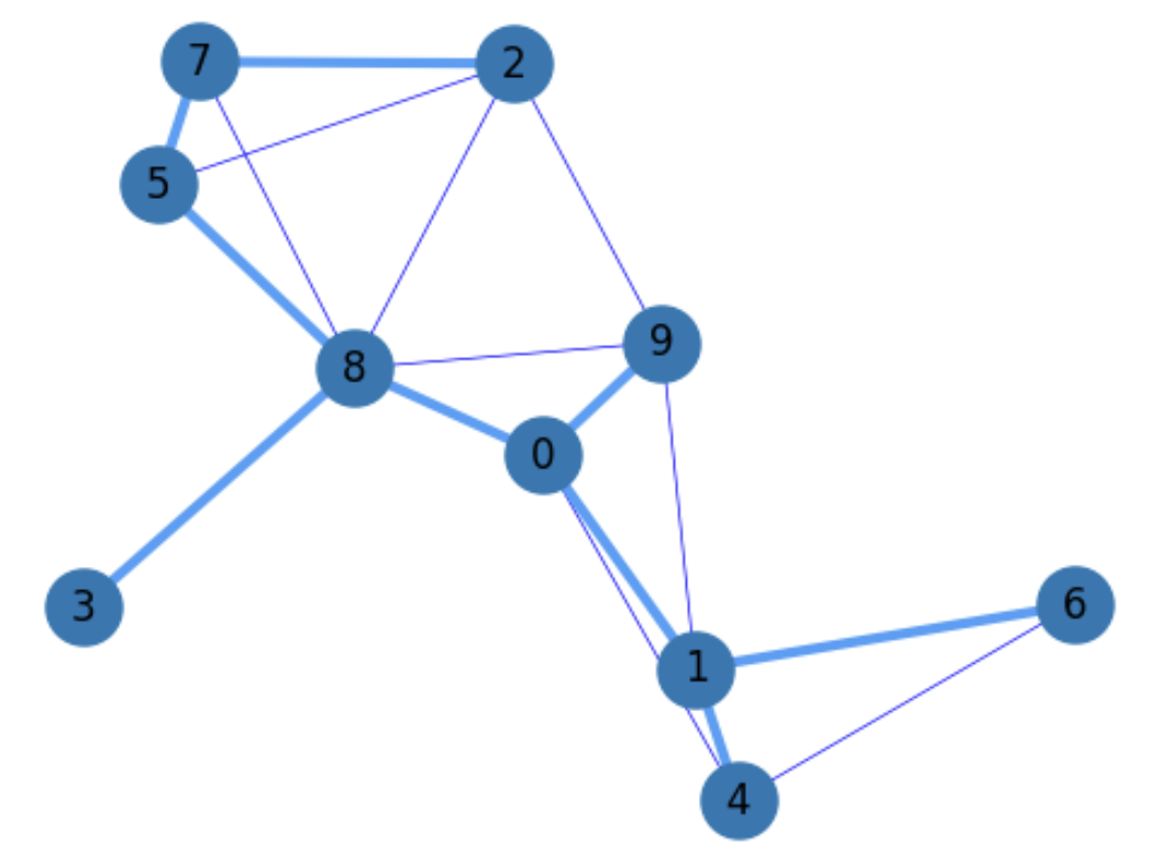
_images/TSP2.png — Fig. 5.19 TSP Phase 1: Compute a MST.#

Concerning the TSP problem, the purpose of finding an MST is actually to find an initial way of connecting all the nodes in \(G\) with minimal cost. Of course, this is not a cycle as we can see in TSP2, since th TSP is acyclic, but the Christophides algorithm extends the TSP to find a Hamiltonian cycle in the steps to follow.

5.3.1.2. Min-weight Perfect Matchings#

Given an undirected graph \(G=(V,E)\), a matching \(M\) is a set of non-adjacent edges \(E'\subseteq E\) which do not form loops. As a result:

The edges in \(M\) do not share common nodes.
The matching \(M\) is called maximal if it is not included in any other matching.
The matching \(M\) is called perfect if it links all the nodes in \(G\).
The Min-weight perfect matchings is the perfect matching with minimum total weight \(\sum_{e'\in M}w(e')\). This problem can be solved by the dual of the Edmond’s Blossom Algorithm with complexity \(O(|V|^3)\) by first replacing the weights as follows \(w'(e)=(\max\{w(e):e\in E\}+1)-w(e)\) and then finding the Max-weight perfect matching with the Blossom’s algorithm.

Concerning the MST problem, we exploit the following properties of perfect matchings:

A graph can only contain a perfect matching when the graph has an even number of nodes.
Perfect matchings are always possible in complete graphs such as the one used the TSP. Actually, the number of perfect matchings in the complete graphs (of course with an even number of nodes) is the double factorial of the even number of nodes: \(|V|!!\).

Therefore, before computing the Min-weight Perfect Matching, we remove from \(G\) all the nodes wich have an odd degree in the MST \(T\). Doing so, we obtain edges with the smallest weights as possible. As we show in TSP3, where we add the min-weight perfect matching \(M\), being

\[ M = \{(3, 8), (4, 1), (9, 2), (0, 6)\} \]

we get edges incident in the MST.

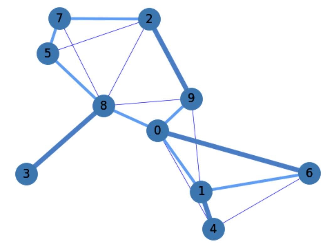
_images/TSP3.png — Fig. 5.20 TSP Phase 2: Add min-weight Perfect Matching to MST.#

5.3.1.3. Eulerian Cycles#

Eulerian cycles (circuits or tours) are cycles where each vertex in the graph is visited once. When the graph is undirected, we consider \((u,v)\neq (v,u)\). Therefore in the above example, we can use \((3,8)\) and \((8,3)\) but not any of them twice!.

The name “Eulerian” comes from the mathematician Leonhard Euler who motivated the problem through the famous Konigsberg-bridges problem. He derived the following necessary condition* for the existence of Eulerian tours in a graph:

Euler’s Theorem. A connected graph has an Euler cycle if and only if every vertex has even degree.

Of course, this condition is satisfied by the TSP graph after removing the vertices with odd degree. Then, a Eulerian tour can be found with complexity \(O(|E|^2)\) with the Fleury’s algorithm.

In particular, the Eulerian tour found by Networkx in the above example is:

\[ \Gamma^0 = 0\rightarrow 6\rightarrow 1\rightarrow 4\rightarrow 1\rightarrow 0\rightarrow 8\rightarrow 3\rightarrow 8\rightarrow 5\rightarrow 7\rightarrow 2\rightarrow 9\rightarrow 0\;. \]

All the edges in \(\Gamma^0\) belong to \(MST\bigcup M\). All we have to do in order to find a Hamiltonian tour is to remove the repeated nodes (shortcult) in \(\Gamma^0\), thus resulting the solution to the MST: