
8. Introduction to the practical part of MD2025#
8.1. Welcome to the practice material of MD2025#
Welcome to the practice part of MD2025. In this part we will learn the main libraries of Python for Machine Learning and Data Science. We will review the main libraries for solving Machine Learning problems, such as Numpy, NetworkX, Matplotlib, Scikit-Learn, etc. We will also learn how to use Jupyter Notebook, a web application that allows you to create and share documents that contain live code, equations, visualizations and explanatory text. The notebooks can be used to perform data cleaning and transformation, numerical simulation, statistical modeling, data visualization, machine learning, etc. In the following code, we will see an example of how to these libraries can work together.
 1import numpy as np
 2import matplotlib.pyplot as plt
 3import networkx as nx
 4
 5np.random.seed(42) # Fijar semilla para reproducibilidad
 6
 7# Crear una matriz de adyacencia aleatoria de 10 x 10
 8A = np.random.randint(0, 2, size=(8, 8))
 9
10# Crear un grafo a partir de la matriz
11G = nx.Graph(A)
12pos = nx.spring_layout(G, seed=42) # Posiciones para graficar [opcional]
13# Dibujar el grafo con matplotlib
14plt.figure(figsize=(10, 8)) # Tamaño del gráfico (ancho, alto)
15plt.title(label='Grafo de ejemplo', # Título
16            fontsize=15, # Tamaño de fuente
17            fontweight='bold', # Tipo de letra
18            color='skyblue', # Color de letra
19            loc='left') # Posición del título
20
21nx.draw(G, with_labels=True, # Mostrar etiquetas
22            pos=pos, # Posiciones
23            node_color='skyblue', # Color de nodos
24            edge_cmap=plt.cm.Blues, # Color de aristas
25            node_size=700,# Tamaño de nodos
26            arrowsize=10, # Tamaño de flechas
27            linewidths=2, # Ancho de aristas
28            font_size=10, # Tamaño de letra de nodos
29            font_weight='bold', # Tipo de letra de nodos
30            font_color='black', # Color de letra de nodos
31            alpha=0.9, # Transparencia
32            width=1) # Ancho de aristas
33plt.show() # Mostrar gráfico
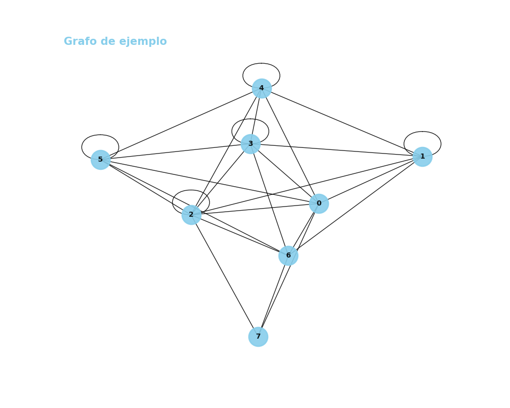
Fig. 8.1 Integration between libraries#
But before we start, we need to set up our environment. For this, we will use Anaconda, a free and open source distribution of the Python and R programming languages for scientific computing, that aims to simplify package management and deployment. Anaconda comes with more than 1,500 packages and a package manager called conda. We will use conda to install the libraries we need for this course.
8.2. Installing Conda#
There are lots of ways to install conda, but we recommend you to install Anaconda. There are lots of tutorials on how to install Anaconda in Youtube or websites. Here are some of them, but again, you can choose the one you like the most. To install Anaconda, you can follow the instructions in the following link: https://docs.anaconda.com/anaconda/install/. Once you have installed Anaconda, you can open the Anaconda Navigator and install the libraries we will use in this course. To do this, you can follow the instructions in the following link: https://docs.anaconda.com/anaconda/navigator/getting-started/.
Warning
After trying your best and spent 2 or 3 hours, if you have any problems installing Anaconda,, you can ask for help by sending an email to the following address: ahmed.begga@ua.es. Please, include the error message you are getting and the steps you have followed to install Anaconda. And do not send trivial questions, please.
8.2.1. Other resources for installing Anaconda#
8.3. IDEs for Python#
You can use any IDE you want to write your code. However, we recommend you to use Jupyter Notebook, a web application that allows you to create and share documents that contain live code, equations, visualizations and explanatory text. The notebooks can be used to perform data cleaning and transformation, numerical simulation, statistical modeling, data visualization, machine learning, etc. To install Jupyter Notebook, you can follow the instructions in the following link: https://jupyter.org/install.
Note
In this course, we will use Jupyter Notebook to write our practical reports. You can use any other IDE you want, but we recommend you to use Jupyter Notebook.
8.3.1. Jupyter Notebook#
Jupyter Notebook is an user-friendly IDE that allows you to write code in Python and Markdown. It is very useful for writing reports, as you can write code and text in the same document. Here we are going to give you few commands to learn how to use markdown in Jupyter Notebook. For more information, you can check the following link: jupyter tutorial.
8.3.1.1. Headers#
To create a header, you can use the following syntax:
# Header 1
## Header 2
### Header 3
#### Header 4
##### Header 5
###### Header 6
8.3.1.2. Emphasis#
To create emphasis, you can use the following syntax:
*italic*
**bold**
***bold and italic***
~~strikethrough~~
8.3.1.3. Lists#
To create lists, you can use the following syntax:
- Item 1
- Item 2
- Item 3
Giving as a result:
Item 1
Item 2
Item 3
You can also create ordered lists:
1. Item 1
2. Item 2
3. Item 3
Giving as a result:
Item 1
Item 2
Item 3
8.3.1.4. Math#
To create math expressions, you can use the following syntax:
$y = x^2$
Giving as a result: \(y = x^2\)
8.3.1.4.1. Math blocks#
To create math blocks, you can use the following syntax:
$$
y = x^2
$$
Giving as a result: $\( y = x^2 \)$
8.3.1.4.2. Math symbols#
To create math symbols, you can use the following syntax:
$\alpha$
$\beta$
$\gamma$
$\delta$
$\epsilon$
$\zeta$
$\eta$
$\theta$
$\iota$
$\kappa$
$\lambda$
$\mu$
$\nu$
$\xi$
$\pi$
$\rho$
$\sigma$
$\tau$
$\phi$
Giving as a result: \(\alpha, \beta,\gamma ,\delta ,\epsilon ,\zeta ,\eta ,\theta ,\iota ,\kappa ,\lambda ,\mu ,\nu ,\xi ,\pi ,\rho ,\sigma ,\tau ,\phi\)
8.3.1.4.3. Matrices#
To create matrices, you can use the following syntax:
$
\begin{bmatrix}
1 & 2 & 3 \\
4 & 5 & 6 \\
7 & 8 & 9
\end{bmatrix}
$
Giving as a result: \( \begin{bmatrix} 1 & 2 & 3 \\ 4 & 5 & 6 \\ 7 & 8 & 9 \end{bmatrix} \)
8.3.1.4.4. Derivatives#
To create derivatives, you can use the following syntax:
$
\frac{dy}{dx}
$
Giving as a result: \( \frac{dy}{dx} \)
8.3.1.4.5. Integrals#
To create integrals, you can use the following syntax:
$
\int_{a}^{b} x^2 dx
$
Giving as a result: \( \int_{a}^{b} x^2 dx \)
8.3.1.4.6. Limits#
To create limits, you can use the following syntax:
$
\lim_{x \to \infty} x^2
$
Giving as a result: \( \lim_{x \to \infty} x^2 \)
8.3.1.4.7. Sums#
To create sums, you can use the following syntax:
$
\sum_{i=1}^{n} x_i
$
Giving as a result:
\( \sum_{i=1}^{n} x_i \)
8.3.1.4.8. Products#
To create products, you can use the following syntax:
$
\prod_{i=1}^{n} x_i
$
Giving as a result: \( \prod_{i=1}^{n} x_i \)
8.3.1.4.9. Roots#
To create roots, you can use the following syntax:
$
\sqrt{x}
$
Giving as a result: \( \sqrt{x} \)
8.3.1.4.10. Fractions#
To create fractions, you can use the following syntax:
$
\frac{1}{2}
$
Giving as a result: \( \frac{1}{2} \)
8.3.1.5. Tables#
To create tables, you can use the following syntax:
| Header 1 | Header 2 |
| -------- | -------- |
| Cell 1   | Cell 2   |
| Cell 3   | Cell 4   |
Giving as a result:
Header 1 |
Header 2 |
|---|---|
Cell 1 |
Cell 2 |
Cell 3 |
Cell 4 |
8.3.1.6. Images#
To add an image, you can use the following syntax:

8.3.1.7. Links#
To add a link, you can use the following syntax:
[link text](url)
8.3.1.8. Citations#
We have agreed to add them by hand with bullets like this:
- [1] Author, Title, Year
- [2] Author, Title, Year