
19. Real cases part 2: Into the Message Passing and Graph Classification#
In this section, we will explore the message passing and graph classification tasks. We will use the same dataset as in the previous section and we will add a new dataset to explore the graph classification task. This new dataset is MUTAG, which is a dataset of chemical compounds. The goal is to predict whether a molecule is mutagenic or not. The dataset is available in the torch_geometric.datasets module.
19.1. Message Passing#
In the previous section, we have seen how to use node2vec to generate node embeddings. In this section, we will use the message passing (not neural message passing) to generate node embeddings. The message passing is a technique to propagate information between nodes in a graph. The message passing is a fundamental concept in graph neural networks.
The message passing is defined as follows:
Each node sends a message to its neighbors.
Each node aggregates the messages from its neighbors.
Each node updates its own state based on the aggregated messages.
In a mathematical form, the message passing can be defined as follows:
where \(h_v^{(l)}\) is the state of node \(v\) at layer \(l\), \(\mathcal{N}(v)\) is the set of neighbors of node \(v\), and \(\text{AGGREGATE}^{(l)}\) is the aggregation function at layer \(l\). The aggregation function can be a sum, mean, max, etc. If we use the sum aggregation function, the message passing can be defined as follows:
And in matrix form, the message passing can be defined as follows:
where \(H^{(l)}\) is the state matrix at layer \(l\), \(A\) is the adjacency matrix, and \(H^{(l+1)}\) is the state matrix at layer \(l+1\). The message passing can be applied multiple times to generate node embeddings. The node embeddings can be used for node classification, link prediction, etc.
19.1.1. Message Passing for Node Classification#
In this section, we will use the message passing for node classification. We will use the Cora dataset. The Cora dataset is a citation network. The nodes represent papers and the edges represent citations. The goal is to predict the category of each paper. The categories are Case_Based, Genetic_Algorithms, Neural_Networks, Probabilistic_Methods, Reinforcement_Learning, and Theory. The dataset is available in the torch_geometric.datasets module.
Let’s start by loading the Cora dataset using Pytorch Geometric.
import torch
from torch_geometric.datasets import Planetoid # Pytorch Geometric datasets
import torch_geometric.transforms as T # Pytorch Geometric transformations, in this case we are going to use the LargestConnectedComponents
from torch_geometric.utils import to_networkx # Convert PyG data object to NetworkX graph

# Load the Cora dataset
# root: root directory where the dataset should be saved
# name: name of the dataset
# transform: a function/transform that takes in an optional argument and returns a transformed version
dataset = Planetoid(root='data/Cora', name='Cora', transform=T.LargestConnectedComponents())
# Get the first element of the dataset, since it is a list of PyG data objects
data = dataset[0]
# Convert the PyG data object to a NetworkX graph
G = to_networkx(data, to_undirected=True)
# Get the labels of the nodes
labels = data.y.numpy()
print(f'Number of nodes: {G.number_of_nodes()}')
print(f'Number of edges: {G.number_of_edges()}')
print(f'Number of classes: {len(set(labels))}')
The code above loads the Cora dataset using Pytorch Geometric and converts it to a NetworkX graph. We then print the number of nodes, edges, and classes in the graph. Now let’s visualize the graph using NetworkX.
import matplotlib.pyplot as plt
plt.figure(figsize=(20, 15))
plt.title('Cora Dataset', fontsize=20)
pos = nx.kamada_kawai_layout(G)
# Color is based on data.y
colors = data.y.numpy()
nx.draw(G, pos=pos, cmap=plt.cm.viridis, node_color=colors, node_size=50, edge_color='black', width=0.7, with_labels=False, node_shape='o', alpha=0.8)
plt.show()
Giving us the following graph:
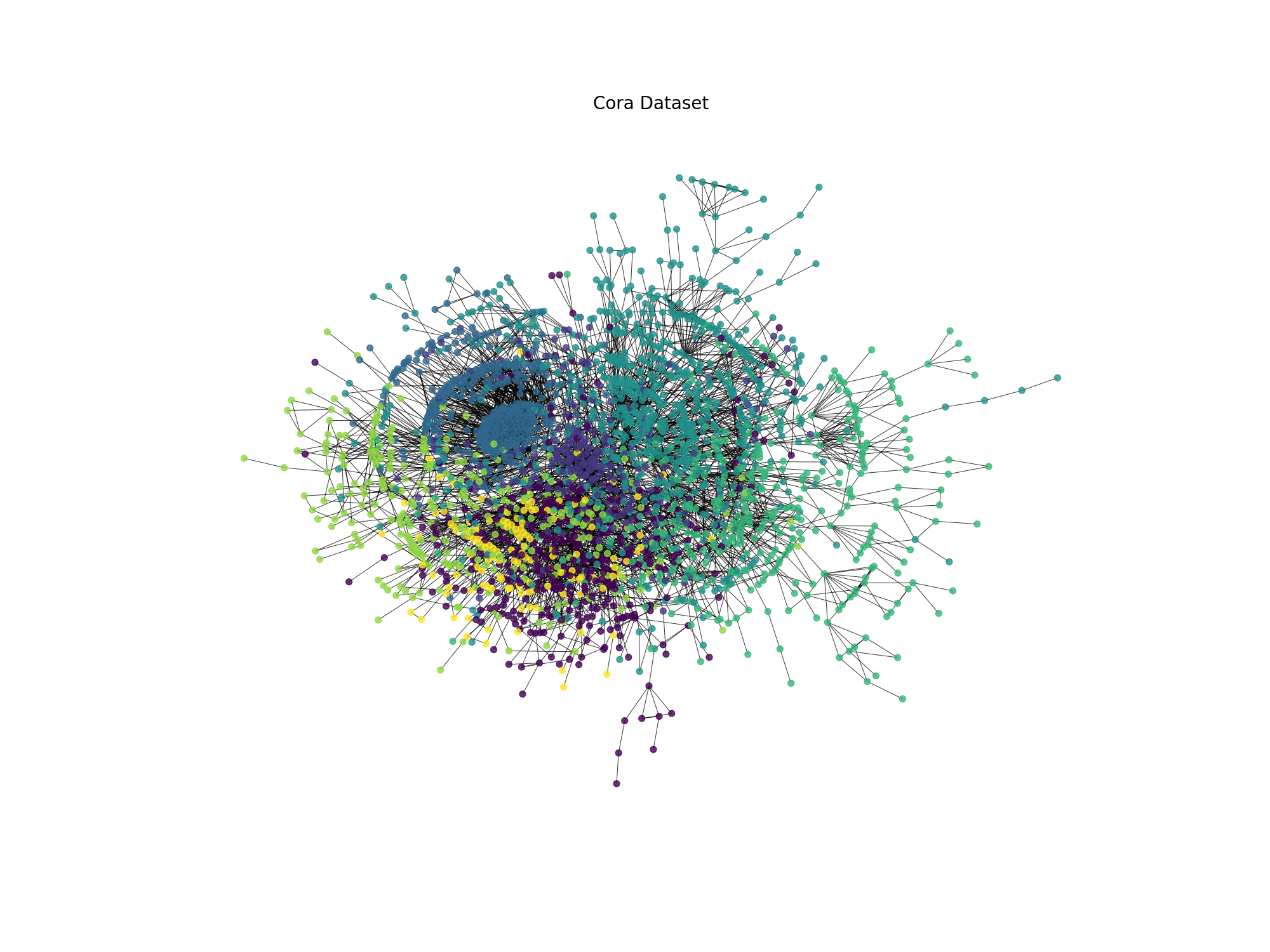
Fig. 19.2 Cora dataset visualization#
The graph represents the Cora dataset, where each node is colored according to its class label. The graph is a citation network, where nodes represent scientific publications and edges represent citations between publications. The colors represent the research areas of the publications.
19.2. Exercises#
19.2.1. Exercise 1#
In the previous section, we learned how to use Node2Vec to generate node embeddings for a graph. Now, we will use the node embeddings of the message passing to perform node classification on the Cora dataset. We will train a simple logistic regression classifier on the node embeddings to predict the class labels of the nodes.
The steps to perform node classification are as follows:
Generate node embeddings using Message Passing.
Train a logistic regression classifier on the node embeddings. Note that you will need to split the dataset into training and test sets (60% training, 40% test).
Evaluate the classifier on the test set. You will need to run the training and evaluation 10 times and calculate the average accuracy to get a more reliable estimate of the classifier’s performance. If you don’t do this, you will get a 0 in the exercise.
Report the average accuracy of the classifier, and discuss the results. In the discussion, I want to see all the parameters that you modified during the process (e.g., the number of time you perform message passing) and how they affected the performance of the classifier. If you put a very long explanation of the parameters that you modified and how they affected the performance of the classifier, you will get a 10 in the exercise, without taking into account the accuracy of the classifier. Important: You need to save the accuracy of each run in a csv file called
node_classification_results_mp_yourname.csvand upload it to the platform. The file should have the following columns:Number_of_message_passing,Accuracy,std. And atleast 3 different configurations of the number of message passing.
IMPORTANT: at least try to perform the message passing 3 times, for instance an experiment with just one message passing, another with 2 and another with 3. Note that the first message passing is \(H^{(1)} = A H^{(0)}\), the second is \(H^{(2)} = A H^{(1)}\) and the third is \(H^{(3)} = A H^{(2)}\), where \(H^{(0)}\) is the initial node features, data.x.
Note
Important: It is forbidden to change the classifier model. Also it is important to initialize the classifier with different random states each time you run the training and evaluation to ensure that the classifier is trained on different data each time. If you don’t do this, you will get a 0 in the exercise.
You can use the following code as a reference:
# Now let's try to classify the nodes using the embeddings
from sklearn.model_selection import train_test_split
from sklearn.linear_model import LogisticRegression
from sklearn.metrics import accuracy_score
# Split the data into training and test sets
X = embeddings
y = data.y.numpy()
X_train, X_test, y_train, y_test = train_test_split(X, y, test_size=0.4, random_state=0)

# Train a logistic regression classifier
clf = LogisticRegression(max_iter=1000, random_state=0)
clf.fit(X_train, y_train)

# Evaluate the classifier
y_pred = clf.predict(X_test)
accuracy = accuracy_score(y_test, y_pred)
print(f'Accuracy: {accuracy:.2f}')
19.2.2. Exercise 2#
In the previous section, we learned how to use node2vec and in this section, we learned how to use the message passing to generate node embeddings. Now, we will combine the node2vec and message passing to generate node embeddings. You just have to concatenate the node embeddings generated by node2vec and message passing. Then, you will train a logistic regression classifier on the concatenated node embeddings to predict the class labels of the nodes. You need to follow the same steps as in Exercise 1.
Important: What I want to see in the discussion is how the combination of node2vec and message passing affected the performance of the classifier. It is also important to mention that is just one experiment, you don’t need to run all the configurations as we did before.
19.3. Graph Classification#
In this section, we will explore the graph classification task. We will use the MUTAG dataset. The MUTAG dataset is a dataset of chemical compounds. The goal is to predict whether a molecule is mutagenic or not. The dataset is available in the torch_geometric.datasets module.
Let’s start by loading the MUTAG dataset using Pytorch Geometric.
import torch
from torch_geometric.datasets import TUDataset
import torch_geometric.transforms as T
from torch_geometric.utils import to_networkx

# Load the MUTAG dataset
dataset = TUDataset(root='data',name='MUTAG')
print(dataset)
print("Number of graphs: ", len(dataset))
print("Number of features: ", dataset.num_features)
print("Number of classes: ", dataset.num_classes)
# Load the first graph in the dataset
data = dataset[0]

print(f'Number of nodes: {G.number_of_nodes()}')
print(f'Number of edges: {G.number_of_edges()}')
print(f'Number of classes: {len(set(labels))}')
The code above loads the MUTAG dataset using Pytorch Geometric and prints the number of graphs, features, and classes in the dataset. Now let’s visualize the first and the fifth graph in the dataset using NetworkX.
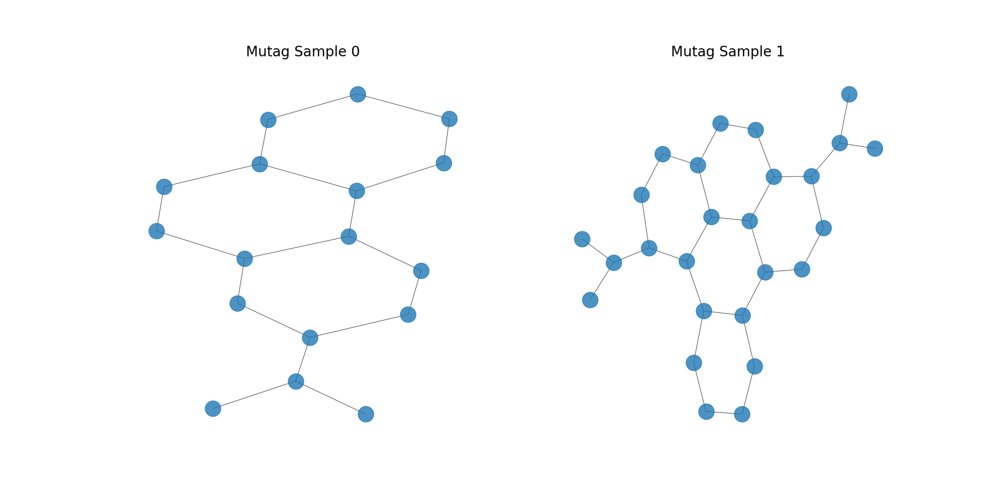
Fig. 19.3 MUTAG#
19.4. Graph2Vec#
In previous sections, we have seen how to generate node embeddings using node2vec and message passing. In this section, we will see how to generate graph embeddings using Graph2Vec. It is similar to node2vec, but instead of generating node embeddings, it generates graph embeddings. How we can generate graph embeddings using Graph2Vec? We only need to create a new embedding containing all the node embeddings of the graph. But, it is important to note that the order of the nodes in the embedding is not important, therefore we need to use a permutation-invariant function to generate the graph embedding. A permutation-invariant function is a function that returns the same output regardless of the order of the input. One example of a permutation-invariant function is the sum function. We can use the sum function to generate the graph embedding. The sum function sums all the node embeddings of the graph to generate the graph embedding.
19.4.1. Steps to generate graph embeddings using Graph2Vec:#
Generate node embeddings using node2vec.
Sum or average the node embeddings to generate the graph embedding.
Use np.vstack to concatenate all the graph embeddings.
19.5. Extra Exercises#
19.5.1. Extra Exercise 1#
In the previous section, we learned how to generate graph embeddings using Graph2Vec. Now, we will use the graph embeddings to perform graph classification on the MUTAG dataset. We will train a simple logistic regression classifier on the graph embeddings to predict whether a molecule is mutagenic or not.
The steps to perform graph classification are as follows:
Generate graph embeddings using Graph2Vec.
Train a logistic regression classifier on the graph embeddings. Note that you will need to split the dataset into training and test sets (80% training, 20% test).
You can use the following code as a reference:
from sklearn.model_selection import train_test_split
from sklearn.linear_model import LogisticRegression
from sklearn.metrics import accuracy_score
# Split the data into training and test sets
X = embeddings # If you understand the code above, your embeddings should have the shape (number of graphs, embedding dimension), for example, (188, 16), where 188 is the number of graphs and 16 is the embedding dimension
y = dataset.y.numpy()

X_train, X_test, y_train, y_test = train_test_split(X, y, test_size=0.2, random_state=0)

# Train a logistic regression classifier
clf = LogisticRegression(max_iter=1000, random_state=0)
clf.fit(X_train, y_train)

# Evaluate the classifier
y_pred = clf.predict(X_test)
accuracy = accuracy_score(y_test, y_pred)
print(f'Accuracy: {accuracy:.2f}')
Important: You have to run the training and evaluation 10 times and calculate the average accuracy to get a more reliable estimate of the classifier’s performance. If you don’t do this, you will get a 0 in the exercise.
19.6. Submission#
For the delivery of the practice 4, what you will be asked to do is to make a zip (name_name.zip) containing 4 notebooks: a first notebook containing Graphs on real life section, a second notebook containing Real cases dataset, a third notebook containing the Real cases part 2: Into the Message Passing and Graph Classification and a fourth notebook containing the Extra exercises.
At the end the zip should be like this when you unzip it:
name_name.zip
├── Graphs_on_real_life.ipynb # ALL THE VISUALIZATIONS SHOULD BE AVAILABLE TO SEE, DO NOT FORGET TO EXECUTE ALL THE CELLS
├── Real_cases_dataset.ipynb
    ├── node_classification_results_yourname.csv
├── Real_cases_part2.ipynb
    ├── node_classification_results_mp_yourname.csv
    ├── node_classification_results_mp_node2vec_yourname.csv # Only contains one row with the results of the experiment of the combination of node2vec and message passing
└── Extra_exercises.ipynb
    ├── graph_classification_results_yourname.csv # Only contains one row with the results of the experiment of the graph classification