4. Game Search#
4.1. Pacman#
Motivation. The classical Pacman game illustrates how game playing algorithms work. Basically, a game is a combat between our agent and another one (or more) agents. The rules of this combat are as following (see Chapter 8 in Pearl’s book: ”Heuristics: Intelligent Search Strategies for Problem Solving”):
In principle, there are two adversarial players who alternate in turn, each viewing in the failure of the opponent its own success.
The players have perfect information. This means that the rules are known for each player and there is no room for chance. Each player has complete information about its opponent’s position and the choices available to it.
The game starts at an initial state and ends at a state where using a simple criterion can be declared a WIN, a LOSS or a DRAW.
In Pacman (see Fig. 4.1) the yellow agent is completely aware of the positions of the food and the ghosts at any time. It is also aware of the state of the ghosts (their color moves to white when they become vulnerable). The game ends either when the yellow agent (say YA) eats all the food (WIN) or it is caught by any of the ghosts (LOSS). There is no DRAW in Pacman but there is in other strategy games such as Chess.
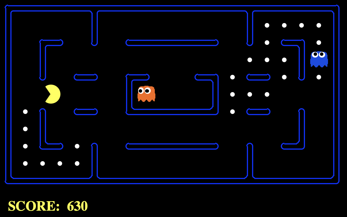
Fig. 4.1 Pacman agent playing against two ghosts. Source: The Berkeley Pac-Man Projects#
4.2. Minimax Adversarial Search#
4.2.1. Game Trees#
A game tree is a state-based representation of all possible plays of the game (see Fig. 4.2):
The root node is the initial position of the game.
The successors of the root are the positions that the first player can reach in one movement.
The respective successors are the positions resulting from the second player’s replies and so on. First and second player levels alternate.
The leaves or terminal nodes of the tree are game ending with WIN, LOSS or DRAW.
Any path from the root to a leaf represent a different complete play of the game.
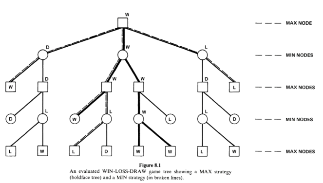
Fig. 4.2 Min-Max game tree with two adversarial players. Source: Pearl’s book.#
The two adversarial players are named MAX and MIN. MAX players are represented by squares \(\square\), and MIN ones with circles \(\bigcirc\).
The tree in Fig. 4.2 shows that MAX can win the play even if MIN do its best. Why? Well, to start with, initially the labels L, W and D are only available at the leaves. They climb to the root as follows:
MIN nodes seek making the MAX player LOOSE. As a result, they will choose from the successors the worst game end wrt MAX. For instance, if the successors of a MIN node are L and W, MIN will choose L. If the successors of the MIN node are L and D, MIN will choose L. Between D and W, MIN will chose D. Finally, MIN will choose W if all its successors are W.
MAX nodes seek making the MAX player WIN. As a result, the will choose from the successors the best game end wrt MAX. Summarizing, MAX will choose L if all its successors are L.
This logic is sumarized by a function called \(\text{STATUS}(J)\).
If \(J\) in a non terminal MAX node, then we have:
If \(J\) in a non terminal MIN node, then we have:
The above definition of \(\text{STATUS}\) shows that MAX and MIN do have an inverse AND/OR logic. Note, for instance, that a MAX node WINs if ANY of its successors, whereas the MIN node WINs only in ALL its successors WIN.
Interestingly, \(\text{STATUS}(J)\) is the best terminal status MAX can achieve from position \(J\) if he plays optimally against a perfect oponent (who also plays optimally).
Solving the game tree \(T\) means labeling the root node with WIN, LOSS or DRAW assuming that both opponents play optimally.
4.2.2. Strategies#
What is an strategy? Given the tree \(T\),
A strategy for MAX is a sub-tree \(T^+\) which contains one successor of each non-terminal MAX node of \(T^+\), and all successors of every non-terminal MIN node of \(T^+\). In Fig. 4.2, the MAX strategy is the subtree in bold.
A strategy for MIN is a sub-tree \(T^-\) which contains one successor of each non-terminal MIN node of \(T^-\), and all successors of every non-terminal MAX node of \(T^+\). In Fig. 4.2, the MIN strategy is the subtree in dashed lines.
Not all strategies are winning. In Fig. 4.2, the MAX strategy is a winning one since we can label the root with WIN even if MIN plays optimally. In other words, with current the terminal labeling, MIN cannot stop MAX winning, even playing its best strategy which is in dashed lines.
Of course, the success of a given strategy depends on the labeling of the terminal nodes. If all of them are labeled as LOSS (WIN), there is no chance of MAX (MIN) to win, but this is, by definition, contrary to the spirit of a game.
However, Fig. 4.2, shows an interesting fact concerning strategies. If you take the terminal nodes belonging to \(T^+\) and \(T^-\), respectively, it is easy to check that there is a single common terminal node. In addition, the label of this terminal node determines the result of the game when both players adhere to their optimal strategies!
If we call \((T^+,T^-)\) to this unique common node, and \(s\) is the root, we have:
What’s the meaning of this? Well, if MAX chooses \(T^+\), MIN can only strike back by choosing the least favorable leaf in \(T^+\) which has label \(\min_{T^-}\text{STATUS}(T^+,T^-)\). But note that in Fig. 4.2. all these leaves are W (this is partially why \(T^+\) encodes a winning strategy for MAX). Then if MIN performs \(\min_{T^-}\text{STATUS}(T^+,T^-)\) if will obtain W! The case of MIN is symmetric.
In other words, if you discover a winning stategy it is pointless to reveal it or not to your opponent (see the case of “checkmate in \(x\) steps” in Chess). Computing \(\text{STATUS}(s)\) is more than finding a winning strategy for MAX, it is an optimization procedure for games.
Exercise. Given the tree in Fig. 4.2, replace the current values in the leaves to a) force a DRAW, and b) force a LOSS. Find, in both cases the common node \((T^+,T^-)\).
Answer:
a) Let us name the current values of \(T\)’s leaves as they are found by a depth-first search DFS algorithm (the usual way it is done): top-down and left-to-right. They are (labeled as \(t_{ijk}\) where \(i\) is the number of child of the MAX root, \(j\) is the level, starting at level \(0\) for the root, and \(k\) is the child number):
\(
\begin{align}
\text{1st subtree:}\;\; & t_{121}=W,\;\; t_{131}=D,\;\; t_{141}=L,\;\; t_{142}=D\\
\text{2nd subtree:}\;\; & t_{231}=W,\;\; t_{241}=L,\;\; t_{242}=D,\;\; t_{243}=W,\;\;t_{244}=W,\;\; t_{234}=L\\
\text{3rd subtree:}\;\; & t_{341}=L,\;\; t_{342}=W,\;\; t_{332}=D,\;\; t_{322}=L\\
\end{align}
\)
In order to force a draw, we need to place either DRAW or LOSS in ALL the three subtrees. There is yet a D in the first subree, and there is a L in the third subtree. Then, we only need to force either a D or a L in the second (central). In order to do so, set \(t_{231}=L\) or \(t_{231}=D\) instead of its current value \(W\). Actually, this is the leaf node corresponding to \((T^+,T^-)\).
b) In order to force a LOSS, we must force a L in ALL the subtrees. A simple way of doing it is to make \(t_{121}=L\) in the first subtree and set \(t_{231}=L\), the \((T^+,T^-)\) leaf, belonging to the second subtree.
4.2.3. The Minimax Method#
Partial expansions. Expanding the complete game tree is pointless in most of the games due to the combinatorial explosion. Chess requires \(10^{120}\) nodes (takes \(10^{101}\) centuries by generating 3 billion nodes per second). As a result, we have to rely on partial expansions (up to a given number of levels) and then apply an evaluation function \(e(J)\) to the leaves \(J\) of this partial expansion.
Evaluation functions. These are static scores evaluating how good is the state of the game wrt MAX. For instance, in Pacman MAX must maximize its distance (Manhattan) wrt the ghosts while minimizing the distance wrt the food. This is encoded by something like
where \(\text{ghost_distance}(J))\) is the closest Manhattan distance to a ghost, and \(\text{food_distance}(J)\) is the closest Manhattan distance to a food point.
Actually, the default evaluation function of Berkeley’s Pacman is as follows:
where:
\(w_1,\ldots, w_5\) are weights (some of them are negative)
\(\text{score}(J)\) the the positional score due to eating food.
\(\text{capsules_distance}(J)\) is the closest distance to a magic capsule (to make the ghosts edible).
\(\text{scared_ghost_distance}(J)\) closest distance to scared ghosts when applicable.
In addition, there are cases where get WIN (clear the board) or LOSS (captured)!
The Minimax Rule. Expand the MAX-MIN tree up to a number of levels and propagate up the \(e(J)\) values of the leaves \(J\) as follows:
If \(J\) is a leaf, then return \(V(J)=e(J)\).
If \(J\) is a MAX node, return its value \(V(J)\) which is equal to the maximum value of any of its successors.
If \(J\) is a MIN node, return its value \(V(J)\) which is equal to the minimum value of any of its successors.
The Minimax rule is implemented by the following recursive algorithm:
Algorithm 4.1 (MINIMAX)
Input Root MAX node \(J\leftarrow \mathbf{s}\)
Output Optimal Minimax Value \(V(J)\).
if \(J\) is terminal then return \(V(J)=e(J)\).
for \(k=1,2,\ldots, b\):
Generate \(J_k\), the \(k-\)th successor of \(J\)
Evaluate \(V(J_k)\) \(\textbf{[recursive call]}\)
if \(k=1\), set \(CV(J)\leftarrow V(J_1)\)
else:
if \(J\) is MAX then set \(CV(J)\leftarrow \max[CV(J),V(J_k)]\)
if \(J\) is MIN then set \(CV(J)\leftarrow \min[CV(J),V(J_k)]\)
return \(V(J)=CV(J)\)
Note that
We call it by calling to \(V(\mathbf{s})\) where \(\mathbf{s}\) is a MAX node. This triggers a call for each of its successors, which are MIN nodes, until a leaf is reached. The first leftmost leaf (step 2.1.1) provides the first clue of the Minimax value of its parent.
Each internal (not-leave) node updates \(CV\) (current value) left-to-right (i.e. in inorder DFS) as the for loop advances. Once we have \(CV(J_1)\) we get \(V(J_2)\) and update \(CV(J)\) if its proceeds.
Curiously, for Pacman we have a MAX level followed by as many MIN levels as ghosts. Then another MAX level occurs, and so on.
Example. In Fig. 4.3 we show a basic example with \(d=4\) levels (we assume that \(d=0\) is the root).
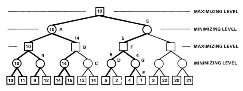
Fig. 4.3 Example of Minimax result with nodes than can been cut. Source: Pearl’s book.#
From Minimax to \(\alpha\beta\). The main limitation of the MINIMAX algorithm is that, in principle we have to span the full subtree until level \(d\) each time it is our turn. In Fig. 4.3, we have that the branching factor is \(b=2\). This implies reaching to \(b^d\) leaves by expanding \(b^0 + b^1 + \ldots + b^{d-1}\) internal nodes.
However, for some arrangements of the evaluation function on the leaves, we may skip nodes to expand by exploiting the assumption that MAX/MIN plays the best it can assuming that the adversary does the same.
Cutoffs. Consider for instance the MIN node \(A\). His leftfost child MAX provides \(10\). Then, as soon as the second one node \(B\) a value equal or greater than \(10\) (\(14\) in this case), we don’t need to expand the subtree rooted in the \(C\). This is an interesting case of cutoff that saves many nodes to expand.
Similarly, once the root receives the value \(10\) from the first child, and proceeds to expand the rightmost subtree, the root will stop such expansion as soon as thid rightmost subtree returs a value smaller or equal than \(10\) (\(5\) in this case). This is another kind of cutoff which is symmetric wrt previous one.
4.2.4. The Alpha-Beta Method#
The above two types or cutoffs or cuts are implemented by the Alpha-Beta algorithm. They are illustrated by the yet classic Fig. 4.4 taken from Pearl’s book.
Let us analize briefly what happens. Shallow cutoff. In Fig. 4.4-Left,
MAX deploys its first level, and its first MIN child A proceeds to deploy its first MAX child which returns \(10\).
Then, MIN knows that the best it can do so far is to choose this move. It keeps going on with its second MAX child.
B receives a value of \(14\). As \(14\ge 10\), MAX knows he had yet beaten MIN.
Then, there is no need to expand more MAX children. This is a cutoff.
Let’s go with the deep cutoff. In Fig. 4.4-Right,
MAX deploys its first child and gets \(10\). This is the best it can do so far.
This value is sent to its second child which is a MIN node.
The value \(10\) reaches MAX node F and its respective child D.
Now D knows that its MAX leaves must play at least equal than \(10\) to be interesting to explore.
However, the first MAX leave returns \(5\), which is very good for MIN since \(5\ge 10\).
Now MIN node D is sure that it will never beat the MAX root if it plays optimally. This is a deep cutoff since no more child of D needs to be explored.
Actually, only a very large value of leave G, say \(20\) may change things, but only in favor of MAX.
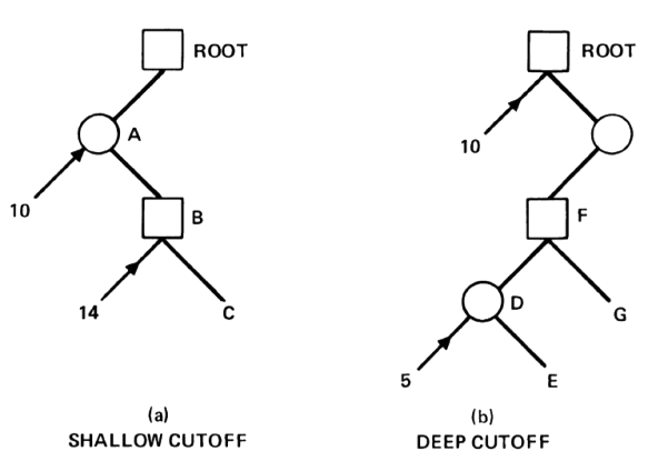
Fig. 4.4 Alpha-Beta cuts. Swallow (leff) vs Deep. Source: Pearl’s book.#
How to put these reasonings in an algorithm. Well, the designers of ALPHA-BETA suggested the following mechanism:
MAX nodes start from \(\alpha=-\infty\) and try to increase that lower bound.
MIN nodes start from \(\beta=+\infty\) and try to decrease that upper bound.
Then, any node (whatever its type) will receive the a pair \((\alpha, \beta)\):
MAX nodes will only update \(\alpha\) and will return \(\beta\) as soon as \(\alpha\ge\beta\). Otherwise they will return \(\alpha\) after exploring their last child.
MIN nodes will only update \(\beta\) and will return \(\alpha\) as soon as \(\beta\le\alpha\). Otherwise they will return \(\beta\) after exploring their last child.
Note that \(\mathbf{\alpha\ge\beta}\) (the cutoff condition) is equal to \(\mathbf{\beta\le\alpha}\) but it is read differently from the perspective of a MAX or a MIN node.
Algorithm 4.2 (ALPHA-BETA)
Inputs Root MAX node \(J\leftarrow \mathbf{s}\), \(\alpha=-\infty\), \(\alpha=+\infty\)
Output Optimal Minimax Value \(V(J)\).
if \(J\) is terminal then return \(V(J)=e(J)\).
for \(k=1,2,\ldots, b\):
Generate \(J_k\), the \(k-\)th successor of \(J\)
if \(J\) is MAX then:
\(\alpha\leftarrow \max[\alpha, V(J_k; \alpha,\beta)]\) \(\textbf{[recursive call]}\)
if \(\alpha\ge\beta\) then return \(\beta\)
if \(k=b\) then return \(\alpha\)
if \(J\) is MIN then:
\(\beta\leftarrow \min[\beta, V(J_k; \alpha,\beta)]\) \(\textbf{[recursive call]}\)
if \(\beta\le\alpha\) then return \(\alpha\)
if \(k=b\) then return \(\beta\)
Algorithm’s trace of the shallow cut
Assign \((-\infty,+\infty)\) to the MAX root.
A node gets \((-\infty,+\infty)\)
A updates its \(\beta\) and sends \((-\infty,10)\) to B.
B updates its \(\alpha\) obtaining \((14,10)\). Since B is a MAX node and \(14\ge 10\), it detects a cut and returns \(\beta=10\).
A still has \((-\infty,10)\) and this is wat returns to the root.
Algorithm’s trace of the deep cut
Assign \((-\infty,+\infty)\) to the MAX root.
The root updates its \(\alpha\) and sends \((10,+\infty)\) to is second child.
The pair \((10,+\infty)\) passes through F and D.
D is a MIN node having \((10,+\infty)\) and it updates its \(\beta\). This leads to \((10,5)\). As \(\beta\le\alpha\), MIN declares a cut and returns its \(\alpha=10\).
F has now the pair \((10,+\infty)\). No cut. It asks G.