8. Graph Matching with Topological Features#
8.1. Practical Session 1.4: Graph Matching with Topological Features#
8.2. Introduction#
In our previous session, we explored basic graph matching using spatial coordinates and the Hungarian Algorithm. While this approach provides a foundation for matching keypoints between images, it only considers geometric distances. In this session, we’ll enhance our matching by incorporating topological features using node2vec and commute times embeddings.
8.3. Theoretical Background#
8.3.1. Node2vec#
Node2vec is an algorithmic framework for learning continuous feature representations for nodes in networks. It maps nodes to a low-dimensional space of features that maximizes the likelihood of preserving network neighborhoods of nodes. The key advantages are:
Captures structural equivalence and homophily
Flexible random walk strategy
Scalable to large networks
8.3.2. Hitting time#
The hitting time of a graph is the expected number of steps that it takes for a random walk to reach a given node in the graph. The hitting time can be used to measure the connectivity of the graph and to find interesting patterns in the graph. This patterns would be more informative than the shortest path or the random walk, since it will give us a more global view of the graph and it is more robust to noise (noise in a graph is the presence of edges that do not follow the general pattern of the graph).
8.4. Enhanced Matching Algorithm#
We’ll modify our previous approach by:
Computing node embeddings using both node2vec and hitting times
Creating a combined similarity matrix using both spatial and topological features
Applying the Hungarian Algorithm to find optimal matches
8.5. Exercise#
In the previous session, we learned about graph construction methods for matching keypoints in images. In this session, we will implement the Hungarian Algorithm to solve the assignment problem in graph matching. We will use the keypoints extracted from images to create a cost matrix and find the optimal assignment of keypoints between two images.
8.5.1. Exercise 1: Enhanced Graph Matching Using Graph Embeddings#
We’ll modify our previous approach by:
Computing node embeddings using both node2vec and hitting times
Creating a combined similarity matrix using both spatial and topological features
Applying the Hungarian Algorithm to find optimal matches
You must use the scipy.optimize.linear_sum_assignment function to solve the assignment problem.
import numpy as np
from PIL import Image
import scipy.io as sio
import matplotlib.pyplot as plt
from scipy.spatial import Delaunay
from scipy.optimize import linear_sum_assignment
import os # Para leer todos los ficheros de la misma carpeta y no hacerlo a mano
import networkx as nx
from gensim.models import Word2Vec # Para hacer el node2vec
def load_and_preprocess_images(img_path1, img_path2, mat_path1, mat_path2):
    """
    Carga y preprocesa pares de imágenes y sus keypoints
    """
    return img1, img2, kpts1, kpts2

def delaunay_triangulation(kpt):
    """
    Generate adjacency matrix based on Delaunay triangulation
    """
    return A

def compute_node2vec_embeddings(G, dimensions=64, num_walks=10, walk_length=30):
    """
    Compute node2vec embeddings for the graph
    """
    return embeddings
def hitting_time(G, start_node, destination_node, num_walks=100):
    """
    Compute the hitting time between two nodes in the graph
    """
    return hitting_time
def compute_hitting_time_matrix(G):
    """
    Compute hitting time matrix for all pairs of nodes
    """
    n = G.number_of_nodes()
    hitting_times = np.zeros((n, n))

    for i in range(n):
        for j in range(i+1, n):
            h_time = hitting_time(G, i, j)
            hitting_times[i,j] = h_time
            hitting_times[j,i] = h_time
    return hitting_times
def enhanced_spatial_matching(kpts1, kpts2, adj_matrix1, adj_matrix2):
    """
    Perform enhanced matching using spatial, hitting time, and node2vec features
    """


    Args:
        kpts1: Array de keypoints del primer grafo (2xN)
        kpts2: Array de keypoints del segundo grafo (2xN)
        adj_matrix1: Matriz de adyacencia del primer grafo (NxN)
        adj_matrix2: Matriz de adyacencia del segundo grafo (NxN)

    Returns:
        matching: Matriz binaria donde matching[i,j]=1 indica correspondencia entre puntos
    Hints:
        - Primero deberás crear una matriz de costes basada en distancias euclidianas,
        cuyo tamaño será (n1, n2) donde n1 y n2 son el número de keypoints en cada grafo.
        - Seguidamente, deberás rellenar dicha matriz con las distancias euclidianas de los keypoints, las distancias/normas de node2vec y finalmente distancias/normas entre el hitting time.
        - A continuación, deberás aplicar el algoritmo húngaro usando la función linear_sum_assignment, que recibe la matriz de costes y devuelve los índices de los puntos emparejados.
        - Finalmente, deberás crear una matriz de matching a partir de los índices obtenidos.

    """
    # Create graphs
    G1 = nx.from_numpy_array(adj_matrix1)
    G2 = nx.from_numpy_array(adj_matrix2)
    print("Computing node2vec embeddings...")
    node2vec_emb1 = compute_node2vec_embeddings(G1)
    node2vec_emb2 = compute_node2vec_embeddings(G2)

    print("Computing hitting time matrices...")
    hitting_times1 = compute_hitting_time_matrix(G1)
    hitting_times2 = compute_hitting_time_matrix(G2)

    # Create cost matrix combining different features
    cost_matrix = np.zeros((n1, n2))

    for i in range(n1):
        for j in range(n2):
            # Spatial distance
            spatial_dist = np.sqrt(np.sum((kpts1[:,i] - kpts2[:,j])**2))

            # Node2vec similarity
            node2vec_dist = np.sqrt(np.sum((node2vec_emb1[i] - node2vec_emb2[j])**2))

            # Hitting time profile similarity
            hitting_profile_dist = np.sqrt(np.sum((hitting_times1[i] - hitting_times2[j])**2))


            # Combine distances with weights
            cost_matrix[i,j] = (
                0.4 * spatial_dist +
                0.3 * node2vec_dist +
                0.3 * hitting_profile_dist
            )

    return matching

def visualize_matching_full(img1, img2, kpts1, kpts2, adj_matrix1, adj_matrix2, matching):
    """
    Visualiza el matching completo entre dos grafos
    """
    # Crear imagen compuesta
    width = max(img1.size[0], img2.size[0])
    height = max(img1.size[1], img2.size[1])
    composite = Image.new('RGB', (width*2, height))
    composite.paste(img1, (0, 0))
    composite.paste(img2, (width, 0))

    plt.imshow(composite)
8.5.2. Exercise 2: Visualize the Optimal Assignment#
Visualize the optimal assignment by connecting the matched keypoints with lines on the images.
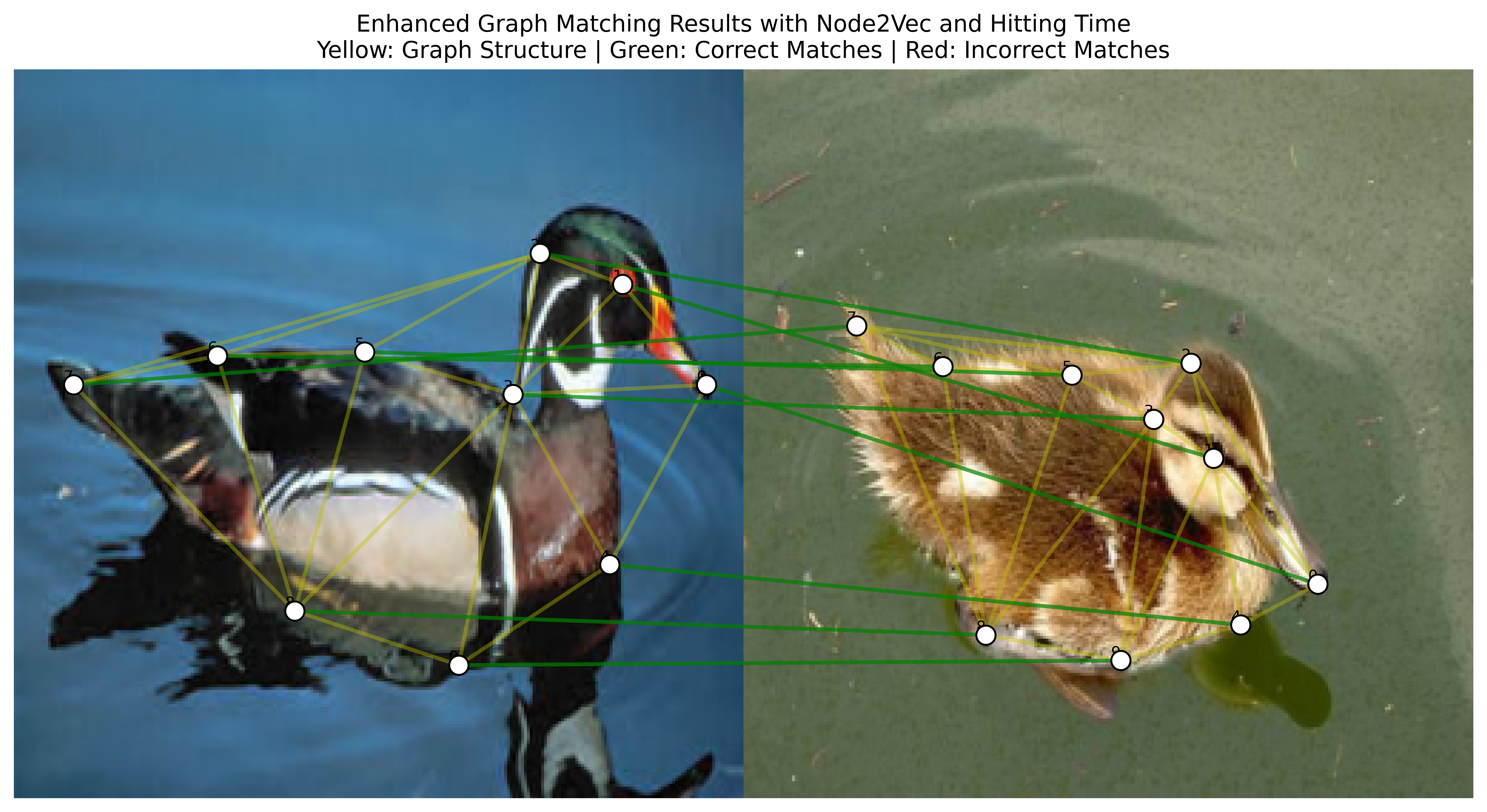
Fig. 8.1 Visualizing the Duck Images with Keypoints,Graph embeddings, Delaunay Triangulation and Matching (Good Result)#
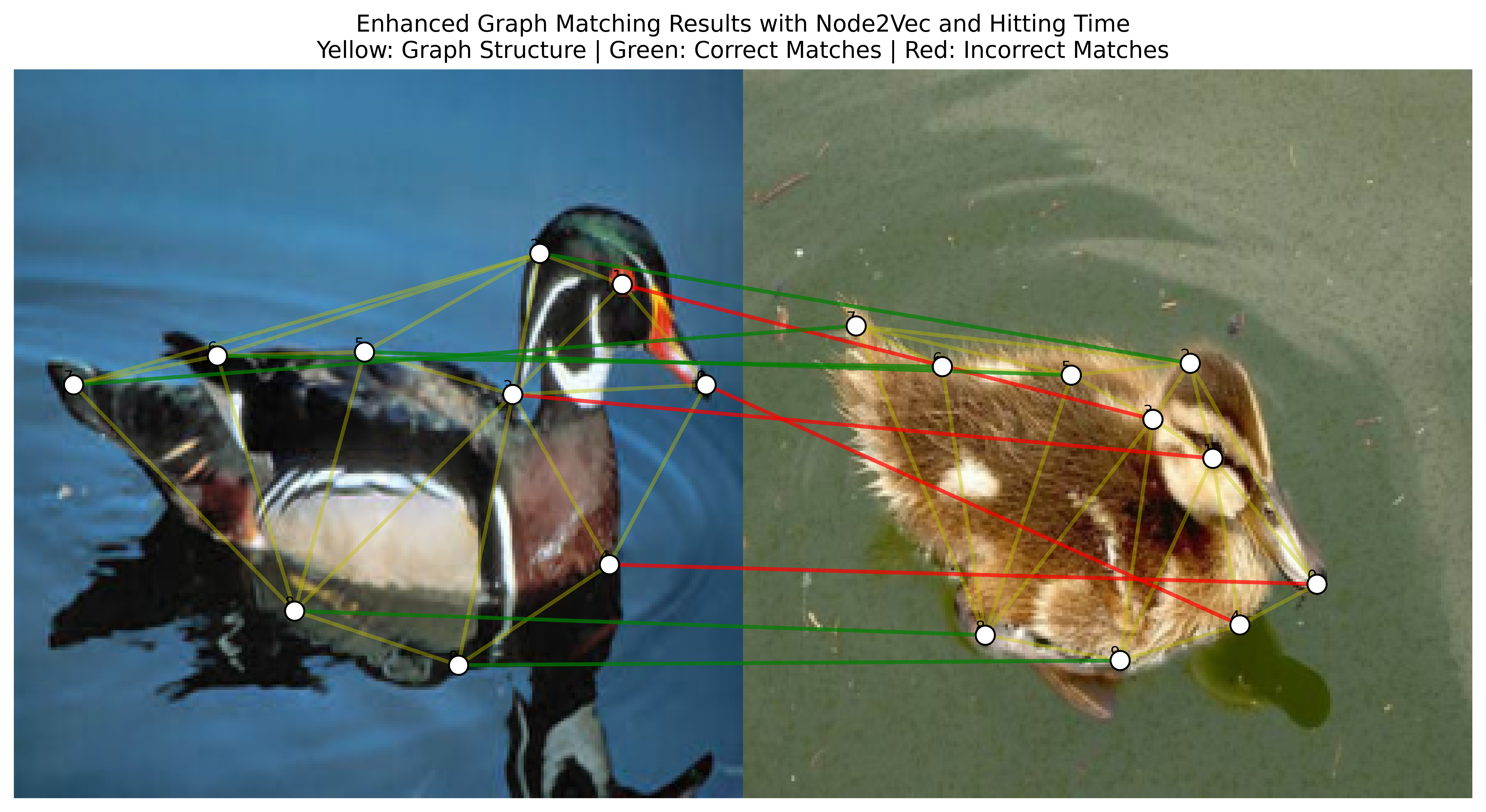
Fig. 8.2 Visualizing the Duck Images with Keypoints,Without Graph embeddings, Delaunay Triangulation and Matching (Bad Result)#
8.5.3. Exercise 3: Evaluate the Matching Results and Report#
Finally, we ask you to extract the accuracy of the matching results. The accuracy is defined as the number of correctly matched keypoints divided by the total number of keypoints. As you know, you have 5 categories of images, so you should evaluate the accuracy for each category, and create a csv file with the results of each category, reporting the mean accuracy for each category and the standard deviation. If you need to perform any other experiment, this is the time to do it.
8.5.4. Exercise 4: Comparative Analysis#
8.5.5. Part 1: Accuracy Analysis Across Categories#
8.5.5.1. Task Requirements#
Calculate matching accuracy for each image category:
Accuracy = (Number of correctly matched keypoints) / (Total number of keypoints)
Process all images in each of the 5 categories
Generate a CSV file containing:
Category name
Mean accuracy
Standard deviation
Number of images processed
8.5.5.2. Expected CSV Format#
Category,Mean_Accuracy,Std_Deviation,Number_of_Images
Category1,0.XX,0.XX,XX
Category2,0.XX,0.XX,XX
...
8.5.6. Part 2: Comparative Analysis#
8.5.6.1. Required Experiments#
Baseline Analysis
Implement spatial-only matching with Delaunay triangulation
Test on all 5 image categories
Record accuracy metrics
Enhanced Matching with Delaunay
Implement enhanced matching (spatial + structural features) using Delaunay triangulation
Test on all 5 image categories
Compare results with baseline
K-Nearest Neighbors Analysis
Select one image category for detailed KNN analysis
Implement and test with:
KNN(3)
KNN(5)
KNN(7)
Compare results with Delaunay triangulation
Weight Sensitivity Analysis
Using your chosen category, experiment with different weight combinations:
Spatial weight: [0.3, 0.4, 0.5, 0.6]
Node2vec weight: [0.2, 0.3, 0.4]
Hitting time weight: [0.2, 0.3, 0.4]
Note: Weights should sum to 1.0
8.5.7. Final Report Requirements#
8.5.8. Format#
Include visualizations (graphs, charts)
Use tables for numerical comparisons
No code needed in the report
8.5.9. Submission format#
name_surname.zip
├── visualization_part_1.ipynb
    └── car.png
    └── face.png
    └── duck.png
    └── motorbike.png
    └── winebottle.png
├── visualization_part_2.ipynb
    └── car_Delaunay.png
    └── face_Delaunay.png
    └── duck_Delaunay.png
    └── motorbike_Delaunay.png
    └── winebottle_Delaunay.png
    └── car_KNN3.png
    └── car_KNN5.png
    └── car_KNN7.png
    └── face_KNN3.png
    └── face_KNN5.png
    └── face_KNN7.png
    └── duck_KNN3.png
    └── duck_KNN5.png
    └── duck_KNN7.png
    └── motorbike_KNN3.png
    └── motorbike_KNN5.png
    └── motorbike_KNN7.png
    └── winebottle_KNN3.png
    └── winebottle_KNN5.png
    └── winebottle_KNN7.png
├── match_part_1.ipynb
    └── results.csv
    └── some_images.png
├── match_part_2.ipynb
    └── results.csv
    └── some_images.png
├── report.ipynb
8.6. Evaluation Criteria#
Your work will be evaluated based on:
Thoroughness of analysis
Quality of visualizations
Clarity of conclusions