13. Assignment 06/25

13.1. SAT3 vs Clique

Exercise Q1. Is the formula \( \underbrace{(x_1\lor x_2\lor \neg x_3)}_{c_1}\land \underbrace{(\neg x_1\lor \neg x_2\lor x_3)}_{c_2} \) satisfiable? Reason about it and show how to decide it by means of reducing SAT3 to Maximal Clique.

Answer. This formula is clearly satisfiable since each variable is true in one clause and false in the other or viceversa. For instance, if \(x_1=1\) in the first clause, then \(\neg x_1=0\) in the second, and the same reasoning is valid for the remaining variables. In other words, we can make \(x_1=1\) and \(x_2=0\) in the first clause, thus satifying \(c_1\), because \(x_1=1\), and also satisfying \(c_2\) since \(\neg x_2 = 1\).

Concerning the mapping of SAT3 to the Maximal Clique, be aware that we have \(2\) clauses \(c_1=(x_1\lor x_2\lor \neg x_3)\) and \(c_2=(\neg x_1\lor \neg x_2\lor x_3)\). Mapping SAT3 to Maximal Clique consists of creating a graph with as many nodes as literals: \(3c\), where \(c\) is the number of clauses. The edges in the clique graph can link any pair of literals except \(x_i\) and \(\neg x_i\). In In Fig. 13.1, we show all the possible edges.

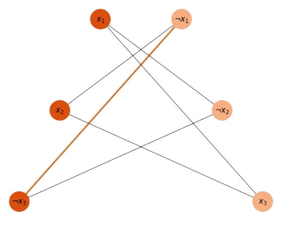
Fig. 13.1 Possible to create many cliques of \(c=2\) nodes.

Once we have the clique graph, if the formula is satisfiable we will find cliques of size \(c\). Since in the above problem, we have \(c=2\), then **any edge in the above clique graph creates a clique of size \(c=2\), in particular \(x_1\) and \(\neg x_2\).

13.2. Graph Matching

Exercise Q2. Given the pair of graphs \(X=(V,E)\) (left) and \(Y=(V',E')\) right in Fig. 13.2, the current assignment encodes a way of making \(X\) a exact subgraph of \(Y\). a) How many ways do we have of making \(X\) an exact subgraph of \(Y\)?

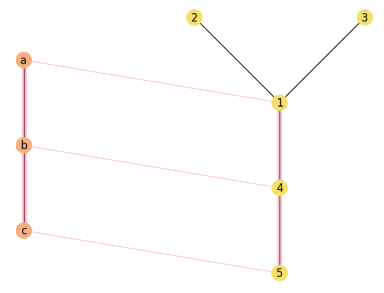
Fig. 13.2 A Maximal Common Substructure.

Answer. Since \(Y\) has \(n=5\) nodes and \(X\) has \(r=3\) nodes, there are \(P(n,r)=n\cdot (n-1)\cdot (n-r+1)\) r-permutations, i.e. \(P(5,3)=5\cdot 4\cdot 3 = 60\) injective mappings \(f_i: V\rightarrow V'\), where \((v\in V, f_i(v)\in V')\). These mappings are order-dependent since they are permutations. As we are asking for Maximum Common Subgraphs (MCS), the only ways of achieving this is to pivoting on assigned notable vertices, i.e. \(b=1\) or \(b=4\), i.e. \((a=\ast,b=1,c=\ast)\) and \((a=\ast,b=4,c=\ast)\). Then, we have the following permutations leading to MCS:


\( \begin{aligned} &\begin{array}{cccc} \text{Subgraph} & \text{Permutation} & \text{Nodes} & \text{Edges}\\ s_1 & f_1=(a=2, b=1, c=3) & V_1'=\{1,2,3\} & E_1'=\{(1,2),(1,3)\}\\ s_2 & f_2=(a=3, b=1, c=2) & V_2'=\{1,2,3\} & E_2'=\{(1,2),(1,3)\}\\ s_3 & f_3=(a=2, b=1, c=4) & V_3'=\{1,2,4\} & E_3'=\{(1,2),(1,4)\}\\ s_4 & f_4=(a=4, b=1, c=2) & V_4'=\{1,2,4\} & E_4'=\{(1,2),(1,4)\}\\ s_5 & f_5=(a=1, b=4, c=5) & V_5'=\{1,4,5\} & E_5'=\{(1,4),(4,5)\}\\ s_6 & f_6=(a=5, b=4, c=4) & V_6'=\{1,4,5\} & E_6'=\{(1,4),(4,5)\}\\ \end{array} \end{aligned} \)

As a result, only \(6/60=10\%\) of the permutations lead to an optimal solution or MCS.

b) What is the formal space of solutions and the cost function to maximize.

Answer. Each candidate assignment \(f:V\rightarrow V'\) is encoded by a binary assignment matrix \(\mathbf{M}\in\{0,1\}^{m\times n}\) with \(m\le n\) and \(m=|V|\), \(n=|V'|\).

However, not every binary matrix of size \(m\times n\) encodes a candidate asignment. Only those whose rows do not have more than \(m\) ones and whose columns do have either a single one or none, encode injective functions, i.e. valid assignments. The solution/search space is given by the set of assignment matrices \({\cal P}\) where,

\( \begin{align} {\cal P}=&\left\{\mathbf{M}\in \{0,1\}^{m\times n}:\forall a\in V:\sum_{i\in V'}\mathbf{M}_{ai}\le 1\;\text{and}\; \forall i\in V':\sum_{a\in V}\mathbf{M}_{ai}\le 1\;\right\}\;. \end{align} \)

Only if \(m=n\), we have that assignment matrices become permutation matrices, i.e. a unique one per row and columb is allowed. Then, the solution space is the Permuthoedron \(\Pi_n\)

\( \begin{align} \Pi_n=&\left\{\mathbf{M}\in \{0,1\}^{n\times n}:\forall a\in V:\sum_{i\in V'}\mathbf{M}_{ai}= 1\;\text{and}\; \forall i\in V':\sum_{a\in V}\mathbf{M}_{ai}= 1\;\right\}\;. \end{align} \)

Concerning the cost function, the most popular is the quadratic assignment function which counts the number of rectangles (if a node \(a\) in \(X\) matches another one \(i\) in \(Y\), then their respective neighbors are enforced to match; otherwise this is not a godd choice). Remember that a rectangle exists if its four sides do exist, i.e. if

\( \exists a,b\in V, \exists i,j\in V':\; \mathbf{M}_{ai}\mathbf{M}_{bj}\mathbf{X}_{ab}\mathbf{Y}_{ij}>0\;, \)

where \(\mathbf{X}_{ab}\) and \(\mathbf{Y}_{ij}\) encode the respective neighboring rules (sides of the rectangle) as we show in Fig. 13.3.

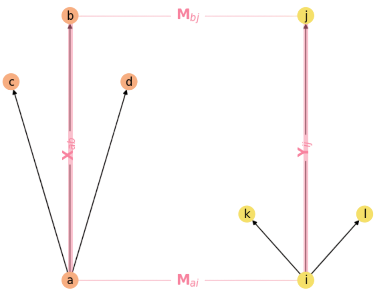
Fig. 13.3 The Rectangle Rule in Graph Matching.

Then the quadratic cost function that counts the number of rectangles closed by \(\mathbf{M}\) is:

\( F(\mathbf{M}) = \frac{1}{2}\sum_{a\in V}\sum_{i\in V'}\sum_{b\in V}\sum_{j\in V'}\mathbf{M}_{ai}\mathbf{M}_{bj}\mathbf{X}_{ab}\mathbf{Y}_{ij}\;, \)

Whose matricial form is

\( F(\mathbf{M}) = \frac{1}{2}\sum_{a}\sum_{i}(((\mathbf{X}\mathbf{M})\mathbf{Y})\odot \mathbf{M})_{ai}\;. \)

c) Propose a random walk in the solution space \({\cal P}\) such as \(\omega_0\rightarrow\omega_1\rightarrow\omega_2\rightarrow\omega_3\) generated by Simulated annealing starting by \(\omega_0=(a=1,b=5,c=2)\). In each case justify the decision taken by SA based on the quadratic cost function.

Answer. SA creates a random walk \(X_0,X_1,\ldots\) on \(\Omega={\cal P}\) through the following Markov chain: \( p(X_{t+1}=\omega'|X_{t}=\omega) = \begin{cases} 1 &\;\text{if}\; \Delta F\ge 0 \\[2ex] \exp(\beta(t)\cdot \Delta F)&\;\text{otherwise}\\[2ex] \end{cases} \)

where \(\Delta F:=F(\omega')-F(\omega)\) and \(\beta(t):=\frac{1}{T(t)}\) where \(T\) is the computational temperature.

1st step. Since \(\omega_0=(a=1,b=5,c=2)\), and the Markov chain must be irreducible (every state in \(\Omega\) must be reachable), the neighbors \(\omega'\in {\cal N}_{\omega_0}\) are defined as follows:

Choose one to variables to change: \(a\), \(b\), \(c\). Say we choose \(b\). This means that \(\omega'\) has the form \((a=1,b=\ast,c=2)\).

Since \(\omega'\) (actually, its matricial representation) must be in \({\cal P}\), we have that \(b\not\in\{1,2\}\). Therefore, \(\omega'\in\{3,4,5\}\). We could repeat \(5\) but we decide (the sampler decides) to pick \(b=4\).

With \(\omega'=(a=1,b=4,c=2)\) we have that \(F(\omega')=1\) since we close a unique rectangle. However, for \(\omega_0=(a=1,b=5,c=2)\) we have \(F(\omega)=0\) (no rectangles). As a result \(\Delta F = 1 - 0 = 1>0\) and this indicates that we must accept \(\omega'\), which (officially) becomes \(\omega_1\).

2nd step. Now, we have \(\omega_1=(a=1,b=4,c=2)\) and we must choice \(\omega'\in {\cal N}_{\omega_1}\) and \(\omega'\in{\cal P}\). One possibility is to make \(a=3\). This results in \(\omega'=(a=3,b=4,c=2)\) which has \(F(\omega')=0\) (zero rectangles). Since \(\Delta F = 0 - 1 < 0\). This configuration is accepted with probability

\( q = \exp(\beta(t)\cdot \Delta F) = \exp\left(\frac{\Delta F}{T(t)}\right) = \exp\left(\frac{-1}{T(t)}\right) \)

We have that \(exp(-1)=\frac{1}{e}=0.37\). This means that for \(T(1)=10\) we have:

\( exp(-1/10)=\frac{1}{exp(1/10)}=\frac{1}{exp(0.1)}=\frac{1}{1.10}=0.9\;. \)

This means that \(p\approx 1\). Then, if we randomnly generate \(p\in [0,1]\) it is quite probable to get \(q=0.9\ge p\). In other words, it is easy to accept \(\omega'\) which becomes the official \(\omega_2\).

3rd step. From \(\omega_2=(a=3,b=4,c=2)\) we can easily select \(b\) and then set \(b=1\) leading to a legal neighbor \(\omega'=(a=3,b=1,c=2)\). This results in \(F(\omega')=2\) and \(\Delta F = 2 - 0 = 2>0\), which is accepted. We thus get, \(\omega_3=(a=3,b=1,c=2)\), an MCS!

13.3. DA Clustering

Exercise Q3. Starting from the corresponding exercise in the first control, we explain the layout in Fig. 13.4.

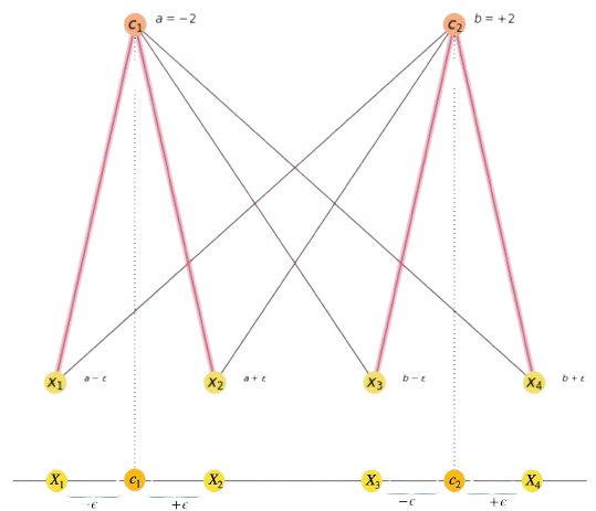
Fig. 13.4 Data-cluster assignment and one-dimensional data layout below.

a) Find a value of \(\epsilon\) which is consistent with the above assignments.

Answer. The image shows a graph-like representation of the one-dimensional layout below. We have four 1D points \(X_1,X_2,X_3\) and \(X_4\). The magenta lines of the graph show that \(X_1\) and \(X_2\) belong to the cluster exemplified by \(c_1\) and \(X_3\) and \(X_4\) belong to the one exemplified by \(c_2\).

For this to be true, we must have that the probabilities \(\langle\mathbf{M}_{ai}\rangle\) satisfy:

\( \begin{align} &\langle\mathbf{M}_{11}\rangle\approx \langle\mathbf{M}_{21}\rangle>0.5\\ &\langle\mathbf{M}_{32}\rangle\approx \langle\mathbf{M}_{42}\rangle>0.5\\ &\forall a\in\{1,2\}:\langle\mathbf{M}_{a1}\rangle> \langle\mathbf{M}_{a2}\rangle\\ &\forall a\in\{3,4\}:\langle\mathbf{M}_{a2}\rangle> \langle\mathbf{M}_{a1}\rangle\\ \end{align} \)

The left side of the two first condititions is due to symmetry (we add or subtract \(\epsilon\) to \(c_i\) to make \(X_i\)).

Limit case. A good strategy to face a problem is to consider the limit case: \(\epsilon=0\). This makes

\( X_1=X_2=c_1=-2\;\;\text{and}\;\;X_3=X_4=c_2=+2\;. \)

However, doing so we have

\( \begin{align} \langle\mathbf{M}_{a1}\rangle &= \frac{e^{-\beta|X_{a}-c_1|}}{e^{-\beta|X_{a}-c_1|}+e^{-\beta|X_{a}-c_2|}} = \begin{cases} 1 &\;\text{if}\; (a=1\lor a=2)\\[2ex] \frac{e^{-\beta|X_{a}-c_1|}}{e^{-\beta|X_{a}-c_1|}+e^{-\beta|X_{a}-c_2|}} &\;\text{otherwise}\:.\\[2ex] \end{cases}\\ \langle\mathbf{M}_{a2}\rangle &= \frac{e^{-\beta|X_{a}-c_2|}}{e^{-\beta|X_{a}-c_1|}+e^{-\beta|X_{a}-c_2|}} = \begin{cases} 1 &\;\text{if}\; (a=3\lor a=4)\\[2ex] \frac{e^{-\beta|X_{a}-c_1|}}{e^{-\beta|X_{a}-c_1|}+e^{-\beta|X_{a}-c_2|}} &\;\text{otherwise}\:.\\[2ex] \end{cases}\\ \end{align} \)

Note that the \(1\)s come from \(e^{-\beta|X_a-c_1|}=1\rightarrow X_a=c_1\), when \(X_a\in\{X_1,X_2\}\), and from \(e^{-\beta|X_a-c_2|}=1\rightarrow X_a=c_2\), when \(X_a\in\{X_3,X_4\}\).

Otherwise, we have the “opposite probabilities”:

\( \begin{align} \langle\mathbf{M}_{31}\rangle &= \frac{e^{-\beta|X_{3}-c_1|}}{e^{-\beta|X_{3}-c_1|}+e^{-\beta|X_{3}-c_2|}} = \frac{e^{-\beta|2-(-2)|}}{e^{-\beta|2-(-2)|}+e^{-\beta|2-2|}}=\frac{e^{-4\beta}}{e^{-4\beta}+1}\\ \langle\mathbf{M}_{41}\rangle &= \langle\mathbf{M}_{31}\rangle\\ \langle\mathbf{M}_{12}\rangle &= \frac{e^{-\beta|X_{1}-c_2|}}{e^{-\beta|X_{1}-c_2|}+e^{-\beta|X{1}-c_1|}} = \frac{e^{-\beta|-2-2|}}{e^{-\beta|-2-2|}+e^{-\beta|2-2|}}=\frac{e^{-4\beta}}{e^{-4\beta}+1}\\ \langle\mathbf{M}_{41}\rangle &= \langle\mathbf{M}_{31}\rangle\\ \end{align} \)

Now, looking at

\( A:=\frac{e^{-4\beta}}{e^{-4\beta}+1}\ll 1\;\text{and}\;\lim_{\beta\rightarrow\infty} A = 0\;. \)

For \(\beta=1\), we have that

\( A(\beta=1):=\frac{e^{-4\beta}}{e^{-4\beta}+1} = \frac{\frac{1}{e^4}}{\frac{1}{e^4}+1} = \frac{\frac{1}{e^4}}{\frac{1 + e^4}{e^4}}=\frac{1}{1 + e^4} = \frac{1}{1 + 54.6}=0.018\;. \)

Therefore, we have:

\( \langle\mathbf{M}\rangle= \begin{bmatrix} 1 & 0.018 \\ 1 & 0.018 \\ 0.018 & 1 \\ 0.018 & 1 \\ \end{bmatrix} \)

Which satisfies the requirement of Fig. 13.4.After normalization, we have

\( \langle\mathbf{M}\rangle= \begin{bmatrix} 0.98 & 0.02 \\ 0.98 & 0.02 \\ 0.02 & 0.98 \\ 0.02 & 0.98 \\ \end{bmatrix}\;. \)

b) Update the centers \(c_i\). This is quite obvious if we apply the correct formula of expectation update.

\( c_i' = \sum_a x_a\frac{\langle\mathbf{M}_{ai}\rangle}{\sum_a \langle\mathbf{M}_{ai}\rangle}\:. \)

Then, considering that \(\sum_a \langle\mathbf{M}_{ai}\rangle\) is the \(i-th\) column of \(\langle \mathbf{M}\rangle\), we have:

\( \begin{align} \sum_a \langle\mathbf{M}_{a1}\rangle &=0.98 + 0.98 + 0.02 + 0.02 = 2\\ \sum_a \langle\mathbf{M}_{a2}\rangle &=0.02 + 0.02 + 0.98 + 0.98 = 2\\ \end{align} \)

Then, we have (looking and the first and second colums of the assignment matrix):

\( \begin{align} c_1' &= \sum_a x_a\frac{\langle\mathbf{M}_{ai}\rangle}{2}=-2\frac{0.98}{2} + -2\frac{0.98}{2} + 2\frac{0.02}{2} + 2\frac{0.02}{2} = -0.98-0.98 + 0.02 + 0.02 = -1.92\\ c_2' &= \sum_a x_a\frac{\langle\mathbf{M}_{ai}\rangle}{2}=-2\frac{0.02}{2} + -2\frac{0.02}{2} + 2\frac{0.98}{2} + 2\frac{0.98}{2} = -0.02-0.02 + 0.98 + 0.98 = +1.92\;.\\ \end{align} \)

Then, all we have is that the centers “approach” eachother:

\( \begin{align} c_1=-2 &\rightarrow c_1'=-1.98\\ c_2=+2 &\rightarrow c_1'=+1.98\:.\\ \end{align} \)

With this analysis to hand, Question Q3 in the exam is quite straight: they ask for update the centers given the assignment matrix

\( \langle\mathbf{M}\rangle= \begin{bmatrix} 0.98 & 0.02 \\ 0.88 & 0.12 \\ 0.12 & 0.88 \\ 0.02 & 0.98 \\ \end{bmatrix}\;. \)

Which is achieved by setting \(\epsilon=1\). Note that, as for \(\epsilon=0\), the new assignment matrix is also consistent with clustering \(X_1\) and \(X_2\) around center \(c_1\) and clustering \(X_3\) and \(X_4\) around center \(c_2\). What is different now is as \(\epsilon\) moves from \(0\) to \(1\), \(X_2\) and \(X_3\) “approach each other” and thus they belong less to their respective cluster!

This explais why, for \(\epsilon=1\), the centers “attract more” each other than with \(\epsilon=0\). If you redo the computations of \(c_1'\) and \(c_2'\) you will obtain:

\( \begin{align} c_1=-2 &\rightarrow c_1'=-1.82\\ c_2=+2 &\rightarrow c_1'=+1.83\:.\\ \end{align} \)

The message to take herein is that as you increment more \(\epsilon\) we have: a) it is more and more likely that \(X_2\) belongs to cluster \(c_2\) since \(X_2 = c_1 + \epsilon\), and b) X_3 belongs to cluster \(c_1\) since \(X_3 = c_2 - \epsilon\) as we show in Fig. 13.5.

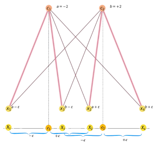
Fig. 13.5 Data-cluster assignment and one-dimensional data layout below.

The configuration depicted in the above figure is just the standard situation where two clusters “intersect”. Finding a theoretical value for \(\epsilon\) is beyond what we answer in the control or exam. However, as in the limit case we may summarize the conditions to be satisfied by the corresponding assignment matrix as follows

\( \begin{align} &\langle\mathbf{M}_{11}\rangle\approx \langle\mathbf{M}_{22}\rangle>0.5\\ &\langle\mathbf{M}_{31}\rangle\approx\langle\mathbf{M}_{42}\rangle>0.5\\ &\forall a\in\{1,3\}:\langle\mathbf{M}_{a1}\rangle> \langle\mathbf{M}_{a2}\rangle\\ &\forall a\in\{2,4\}:\langle\mathbf{M}_{a2}\rangle> \langle\mathbf{M}_{a1}\rangle\\ \end{align} \)

Intuitively, \(\langle\mathbf{M}_{11}\rangle\approx \langle\mathbf{M}_{22}\rangle>0.5\) tells us that

\( \begin{align} &\frac{e^{-\beta |X_1-c_1|}}{e^{-\beta |X_1-c_1|}+e^{-\beta |X_1-c_2|}}\approx \frac{e^{-\beta |X_2-c_2|}}{e^{-\beta |X_2-c_1|}+e^{-\beta |X_2-c_2|}}>\frac{1}{2}\;. \end{align} \)

Keeping in mind the definitions:

\( \begin{align} X_1 &= c_1 - \epsilon\\ X_2 &= c_1 + \epsilon\\ X_3 &= c_2 - \epsilon\\ X_4 &= c_2 + \epsilon\\ \mathbf{c_1} & \mathbf{= - c_2}\\ \end{align} \)

And applying in to the above equations, we have

\( \begin{align} \frac{e^{-\beta |-\epsilon|}}{e^{-\beta |-\epsilon|}+e^{-\beta |2c_1-\epsilon|}} &\approx \frac{e^{-\beta |2c_1 + \epsilon|}}{e^{-\beta |\epsilon|}+e^{-\beta |2c_1 + \epsilon|}}>\frac{1}{2}\;. \end{align} \)

\( \begin{align} \frac{e^{-\beta\epsilon}}{e^{-\beta \epsilon}+e^{-\beta |2c_1-\epsilon|}} &\approx \frac{e^{-\beta |2c_1 + \epsilon|}}{e^{-\beta\epsilon}+e^{-\beta |2c_1 + \epsilon|}}>\frac{1}{2}\;. \end{align} \)

\( \begin{align} \frac{e^{-\beta\epsilon}}{e^{-\beta \epsilon}+e^{-\beta |2(-2)-\epsilon|}} &\approx \frac{e^{-\beta |2\cdot (-2) + \epsilon|}}{e^{-\beta\epsilon}+e^{-\beta |2\cdot (-2) + \epsilon|}}>\frac{1}{2}\;. \end{align} \)

\( \begin{align} \frac{e^{-\beta\epsilon}}{e^{-\beta \epsilon}+e^{-\beta |-4-\epsilon|}} &\approx \frac{e^{-\beta |-4 + \epsilon|}}{e^{-\beta\epsilon}+e^{-\beta |-4 + \epsilon|}}>\frac{1}{2}\;. \end{align} \)

Since \(\epsilon=2\) is the following integer value after \(\epsilon=1\), we update the formulas as follows:


\( \begin{align} \frac{e^{-\beta 2}}{e^{-\beta 2}+e^{-\beta |-4-2|}} &\approx \frac{e^{-\beta |-4 + 2|}}{e^{-\beta 2}+e^{-\beta |-4 + 2|}}>\frac{1}{2}\;. \end{align} \)

And for \(\beta = 1\),

\( \begin{align} \frac{e^{-2}}{e^{-2}+e^{-6}} &\approx \frac{e^{-2}}{e^{-2}+e^{-2}}>\frac{1}{2}\;. \end{align} \)

However, this is not enough since

\( \begin{align} \frac{e^{-2}}{e^{-2}+e^{-2}} = \frac{e^{-2}}{2}=\frac{1}{2e^2}<\frac{1}{2}\;. \end{align} \)

Actually, after computing and normalizing the assignment matrix we have

\( \langle\mathbf{M}\rangle= \begin{bmatrix} 0.98 & 0.02 \\ 0.50 & 0.50 \\ 0.50 & 0.50 \\ 0.02 & 0.98 \\ \end{bmatrix}\;, \)

i.e. \(\langle\mathbf{M}_{21}\rangle = \langle\mathbf{M}_{22}\rangle=1/2\). In other words, for \(\epsilon=2\), \(X_2\) is equidistant from \(c_1\) and \(c_2\).

Consequently, the solution comes with \(\epsilon>2\), in particular, with \(\epsilon=3\) we obtain the following assignment matrix (after normalization):

\( \langle\mathbf{M}\rangle= \begin{bmatrix} 0.98 & 0.02 \\ 0.12 & 0.88 \\ 0.88 & 0.12 \\ 0.02 & 0.98 \\ \end{bmatrix}\;, \) Where \(X_2\) is assigned to cluster \(c_2\) and \(X_3\) to cluster \(c_1\). The centers become:

\( \begin{align} c_1=-2 &\rightarrow c_1'=-2.79\\ c_2=+2 &\rightarrow c_1'=+2.79\:,\\ \end{align} \)

Intrerpretation: as \(X_2\) approaches X_3 and their assigned clusters are twisted, the new centers “diverge” since \(X_1\) and \(X_4\) do also diverge.

13.4. Rubik and Beam Search

Exercise Q4. This is an example of a practical question with a theoretical flavor. All we expect here is that you reason about the heuristic-search procsss. layout in Fig. 13.4.

a) How does BEAM search bound the combinatorial explosion in the Rubik problem.

Answer The Rubik-cube search problem is, as many combinatorial problems, a good example of combinatorial explosion of order \(b^d\), where \(b\) is the branching factor, and \(d\) is depth. Then, if we assume that \(b\) is constant (as it is in Rubik, where \(b=12\)), we expand (by default) the following number of nodes \(S\) (see Iterative-deepening section):

\( S_b = \underbrace{b^0}_{\text{Root=1st level}} + \underbrace{b^1}_{\text{2nd level}} + \underbrace{b^2}_{\text{3rd level}} + \ldots + \underbrace{b^{d}}_{\text{d level}} = \sum_{i=0}^db^i = b^0\left(\frac{1-b^{d}}{1-b}\right)\;. \)

For \(b=2\) we have: \( S_2=\frac{1-2^{d}}{1-2} = -1 + 2^d = 2^d-1\; \)

For \(d=5\) we have: \(2^5 - 1 = 31\) generated nodes as we illustrate Fig. 13.6:

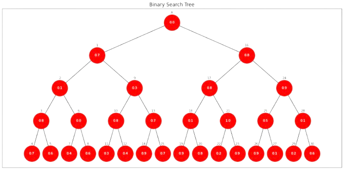
Fig. 13.6 Branching process and combinatorial explosion: \(b=2, d=5\).

The most important issue of combinatorial explosions is that the number of generated nodes is \(O(b^d)\). For Rubik, where \(b=12\) this is unavodable even for modest values of \(d\): For instance, \(12^5 = 249,932\) leads to explore nodes.

BEAM search contains this explosions by allowing to hold the best \(2^k\) (\(k\) is constant) nodes in the OPEN list. Suposse, for instance that \(k=2=b\) in illustrate Fig. 13.6. This means that OPEN can only hold no more that \(2^2=4\) nodes.

First expansion. The number inside a give node is the probability of making this move from the parent according to a deep oracle. As \(g(\mathbf{n})\) is the product of probabilities from the root (we assume \(g(A)=1.0\)), for the first expansion we have \(\text{OPEN}=\{1,16\}\):

\( \begin{align} g(A) &= \mathbf{1.0}\; (\text{not zero because it is the starting point})\\ g(1) &= 1.0\cdot 0.7 = 0.7\\ g(16) &= 1.0\cdot 0.8 = \mathbf{0.8}\\ \end{align} \)

Second expansion. Then, we pick node \(16\) (maximum value) and \(\text{OPEN}=\{1,17,24\}\) whose length is not greater than \(2^2=4\):

\( \begin{align} g(1) &= 1.0\cdot 0.7 = 0.7\\ g(17) &= 1.0\cdot 0.8\cdot 0.8 = 0.64\\ g(24) &= 1.0\cdot 0.8\cdot 0.9 = \mathbf{0.72}\\ \end{align} \)

where the best node to expand is node \(24\). This leads to \(\text{OPEN}=\{1,17,25,28\}\) and then

\( \begin{align} g(1) &= 1.0\cdot 0.7 = \mathbf{0.7}\\ g(17) &= 1.0\cdot 0.8\cdot 0.8 = 0.64\\ g(25) &= 1.0\cdot 0.8\cdot 0.9\cdot 0.5 = 0.36\\ g(28) &= 1.0\cdot 0.8\cdot 0.9\cdot 0.1 = 0.072\;.\\ \end{align} \)

Now, the best node is the shallowest one (node \(1\)). After expanding it, we have \(\text{OPEN}=\{2,9,17,25,28\}\) and now \(|\text{OPEN}|=5>4\) forces us to retain the best (maximal) \(4\) nodes (in bold):

\( \begin{align} g(17) &= 1.0\cdot 0.8\cdot 0.8 = \mathbf{0.64}\\ g(25) &= 1.0\cdot 0.8\cdot 0.9\cdot 0.5 = \mathbf{0.36}\\ g(28) &= 1.0\cdot 0.8\cdot 0.9\cdot 0.1 = \mathbf{0.072}\\ g(2) &= 1.0\cdot 0.7\cdot 0.1 = 0.07\\ g(9) &= 1.0\cdot 0.7\cdot 0.3 = \mathbf{0.21}\\ \end{align} \)

And we “purge” node \(2\). Then, the border becomes \(\text{OPEN}=\{9,17,25,28\}\). As you can see, the fact that \(g(\mathbf{n})\) comes for a product keeps a balance between DFS and BFS. In Fig. 13.7, we illustrate the process. The slashes’ colors show what nodes belong to each of the versions of the search border \(\text{OPEN}\), before purging node \(2\).

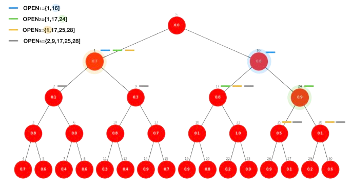
Fig. 13.7 BEAM search in action. Example: \(k=2\).

b,c) How does the deep oracle work? What if all successors are equaly probable?

Answer. At a given node \(\mathbf{n}\), the deep oracle (once trained, i.e. working in the test regimes) provides the proability of each of its succesors: \(b=12\) in Rubik. These are the numbers that we have coded in Fig. 13.7. Remind that in Rubik, each successor is a different move from the configuration coded by \(\mathbf{n}\). Then, \(g(\mathbf{n})\) is calculated as a concatenation of probabilities. Recursively we express this as \(g(\mathbf{n})=p(\mathbf{n})\cdot g(\text{parent}(\mathbf{n}))\) (section “Beam Search and Rubik”).

We have that \(g(\mathbf{n})=\prod_i p(\mathbf{n}_i)\) where \(\mathbf{n}_i\) are all the nodes in the (best) path from \(\mathbf{n}_0\) to \(\mathbf{n}\). In problems such as Rubik, where the configuration space \(\Omega\) is huge, this high-entropy regime is very likely unless we use a vast amount of data to train the deep oracle, as we explain in section “Rubik State Space”. Basically, what happens is that the deep oracle is only “locally effective” and each transition has roughly \(p(\text{successor}(\mathbf{n}))=\frac{1}{12}\). As a result, \(g(\mathbf{n})\approx \frac{1}{12^d}\), where \(d\) is the depth of node \(\mathbf{n}\), and all \(g(\mathbf{n})\) are nearly equal, thus transforming BEAM-search in a constrained BFS. The most entropic the regime, the larger the length of the optimal path (God’s number is \(N=20\) for Rubik). This rationale is summarized in Fig. 13.8.

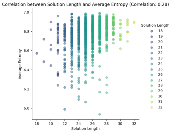
Fig. 13.8 Entropy analysis for many executions of Rubik Beam Search.

In other words, the less entropic (more informative) is the deep oracle, the better. And this often relies on both: a) increasing the size of the training set, b) increasing the \(k\) of \(2^k\) to uncover more alternative paths during BEAM search.

13.5. Alpha-Beta Cuts

Exercise Q5. Typical problem for testing the \(\alpha-\beta\) algorithm in a MINIMAX tree.

a) Solve the a MINIMAX tree, noting the cuts and the saving over MINIMAX.

Answer: we put the solution directly in Fig. 13.9, showing (left-to-right or top-down) the order in which we update \(\alpha\) in MAX nodes and \(\beta\) in MIN nodes, if it proceeds. Put the values returned by the children to be more informative.

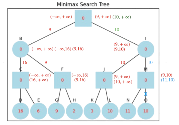
Fig. 13.9 Alpha-Beta algorithm on a MINIMAX tree.

Cuts \(\alpha\ge\beta\) are coded in blue, and the green value is that of the leaf node determining the best choice for the MAX root. Note that in the left part of the tree, the best value is \(9\), but later on, the algorithm discovers \(10\) (right-part of the tree). It is always interesting to identify what leaf node leads to a partial or global solution. We have a single cut and we save only a single node wrt MINIMAX.

b) What should be the value in node \(G\) to create a cut?


Answer: Note that when \((-\infty, 16)\) arrives to \(F\) (\(G\)’s parent), MAX must update its \(\alpha\) (which is \(-\infty\) at the time) so that \(\alpha\ge\beta\) (\(\beta=16\) at the time). As a result, the required value \(X\) should be \(X\ge 16\) to cut \(H\).