2. Simulated and Deterministic Annealing#
2.1. Maximum Common Subgraph#
Motivation. Chemical compounds exhibit structural patters shared between compounds of the same family. One of these patterns is the circular (hexagonal) structure formed by carbon (C) atoms linked by single or double bonds (see Fig. 2.1-Left and Center) where the non-labeled vertices denote C atoms. In this example, the presence of the hexagonal ring in the popular Aspirin (Fig. 2.1-Right) is well known.
The development of AI pattern matching techniques for detetecting substructures has powered the field of Bioinformatics. Nowadays, the analysis of exponentially growing datasets of proteins such as the Protein Data Bank PDB or of chemical compounds such as PubChem is a must in AI.
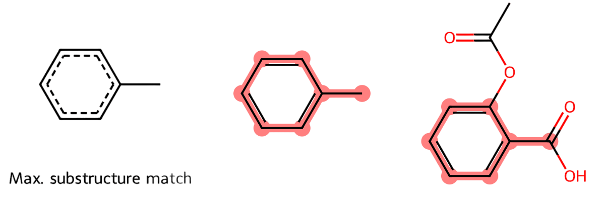
Fig. 2.1 Structure of the Aspirin.#
MCS. Comparing substructures is not an easy problem. Whereas comparing substrings is polynomial, comparing substrutures is a well-known NP problem called the Maximum Common Subgraph or MCS:
Given two graphs \(G_1=(V_1,E_1)\) and \(G_2=(V_2,E_2)\), what is the graph \(H=(V,E)\) that is common to \(G_1\) and \(G_2\) with the maximum number of nodes?
Herein, common means the following: \(V = V\subseteq V_1\) and \(E\subseteq E_1\) and exists an injective (one-to-one) mapping \(f:V\rightarrow V_2\) such that \((i,j)\in E\) iff \((f(i),f(j))\in E_2\).
This subsetness flavor clarifies the fact that \(\text{MCS}\in \text{NP}\). Actually, MCS does not only search for one common subset but for the subset with the maximum number of nodes.
This is quite clear in the following Breaking Bad problem: What is the structural coincidence between Ectasy and Amphetamine?.
According to PubChem, Ectasy is derived from the Amphetamine.
Looking at Fig. 2.2-Center (Ectasy) comes from removing an Hidrogen atom from Amphetamine (Fig. 2.2-Right), adding a carbon and an oxigen-carbon pentagonal cycle.
The MCS is in Fig. 2.2-Left.
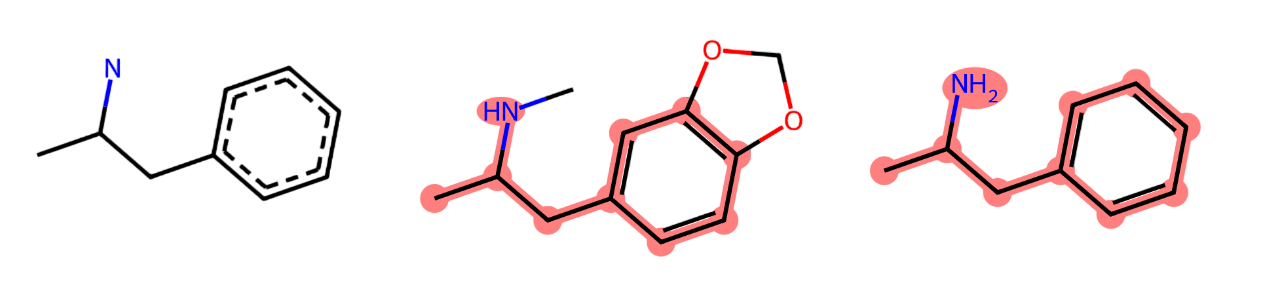
Fig. 2.2 Maximal Common Substructure (left) of two design drugs (center and right).#
All the figures have been generated by the RDKit: Open-Source Cheminformatics Software.
2.2. Graph Matching#
Solving MCS via a polynomial approximation requires finding the injective function \(f\) between the vertices \(V\) of small graph \(X=(V,E)\) and those \(V'\) of larger graph \(Y=(V',E')\) in polynomial time.
2.2.1. Assignments and Matchings#
Node assignments. Consider the (undirected) graphs:
As we have \(n=|V'|=5\) and \(r=|V|=3\) we have \(P(n,r)=n\cdot (n-1)\cdot (n-r + 1)\) r-permutations i.e. one-to-one functions \(f\) or node assignments that can be potential solutions to the MCS problem. In this case, we have \(P(5,3)=5\cdot 4\cdot 3=60\) different assignments. Then, what assignments provide the MCS between \(X\) and \(Y\)?
For the graphs \(X\) and \(Y\) the size of the MCS is \(2\), since \(X\) has only two edges and if it is a subgraph of \(Y\) (as it is really is), the size of the MCS has \(|V|=3\) nodes and |E|=2$ edges.
However, this depends on how good is the injective function \(f\). For the one in Fig. 2.3 we have:
As we can see, \((a,b)\in E\) and \((1=f(a),2=f(b))\in E'\). However, for the other edge \((b,c)\in E\) we have that \((2=f(b),3=f(c))\not\in E'\): As a result \(X\) and \(Y\) do only have one common edge for \(f\) (in magenta).
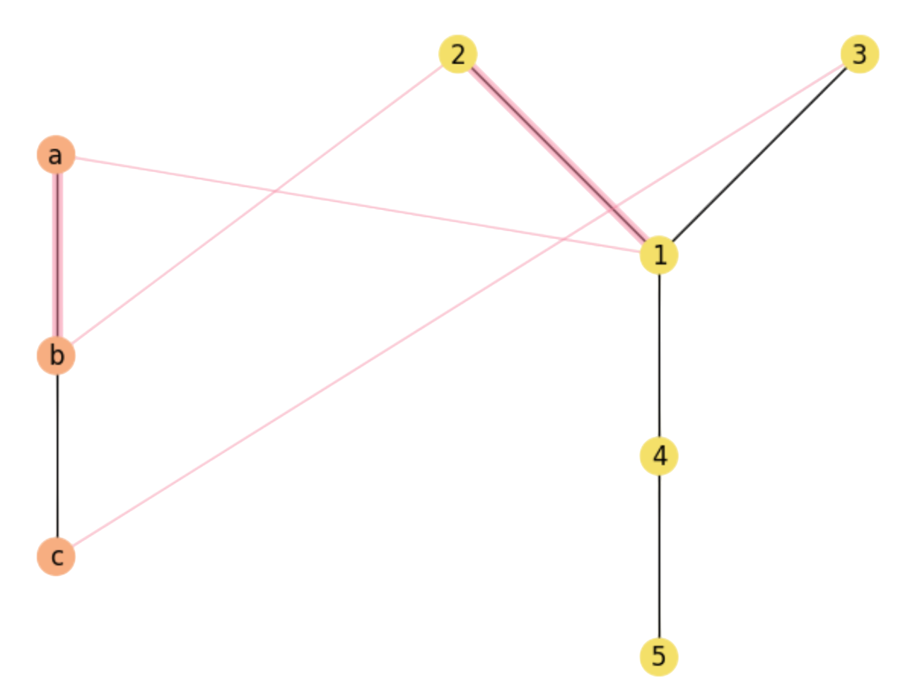
Fig. 2.3 non-Maximal Common Substructure.#
Consider now the assignment:
which indeed leads to a MCS:
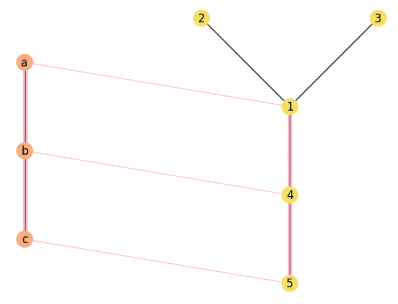
Fig. 2.4 A Maximal Common Substructure.#
However, this MCS assignment is not unique. Actually we have \({5 \choose 3}=10\) subgraphs of \(Y\) where we can embed \(X\) but only \(8\) of them lead to MCS assignments. In the above table, we encode each MCS injective function \(f_i\) as a list of pairwise matchings \((v\in V, f_i(v)\in V')\):
Notable vertices. In the above table, note that MCS assignments usually contain pairwise matchings between nodes with large degrees (notable vertices) in both graphs, namely \(\mathbf{b}\) and \(\mathbf{1}\) or \(\mathbf{4}\) (in bold). These matchings are \(\mathbf{(b,1)}\) and \(\mathbf{(b,4)}\).
In the following exercise we emphasize the link between the subgraphs of \(Y\) and the MCS assignments, which is a fundamental concept in this topic.
Exercise. Identify the \({5 \choose 3}=10\) subgraphs of size \(3\) in \(Y\) (indicating both nodes and edges) and:
a) Detect the ones which do correspond to a complete embedding of \(X\) in \(Y\).b) Identify these subgraphs in the \(8\) MCS assigmnets of the above table.
NOTE. Express always the edges in lexicographical order i.e. \((i,j)\) if \(i<j\).
Answer. a) The subgraphs are the \(10\) combinations of the \(5\) nodes \(V'=\{1,2,3,4,5\}\) in groups of \(3\) nodes (because \(|V|=3\)). However, only those subgraphs wich are connected can lead to a complete embeddding of \(X\) in \(Y\):
\(
\begin{aligned}
&\begin{array}{cclc}
\text{Subgraph} & \text{Nodes} & \text{Edges} & \text{is Connected?}\\
s_1 & V_1'=(1, 2, 3) & E_1'=\{(1,2),(1,3)\} & \checkmark \\
s_2 & V_2'=(1, 2, 4) & E_2'=\{(1,2),(1,3)\} & \checkmark \\
s_3 & V_3'=(1, 2, 5) & E_3'=\{(1,2)\}&\\
s_4 & V_4'=(1, 3, 4) & E_4'=\{(1,3),(1,4)\}& \checkmark\\
s_5 & V_5'=(1, 3, 5) & E_5'=\{(1,3)\}&\\
s_6 & V_6'=(1, 4, 5) & E_6'=\{(1,4),(1,5)\}& \checkmark\\
s_7 & V_7'=(2, 3, 4) & E_7'=\emptyset &\\
s_8 & V_8'=(2, 3, 5) & E_8'=\emptyset &\\
s_9 & V_9'=(2, 4, 5) & E_9'=\{(4,5)\} &\\
s_{10} & V_{10}'=(3, 4, 5) & E_{10}'=\{(4,5)\} &\\
\end{array}
\end{aligned}
\)
b) We have that only subgraphs \(s_1\), \(s_2\), \(s_4\) and \(s_6\) can accomodate the full graph \(X\). In graph theory we say that these subgraphs are isomorphic to \(Y\). Note that each of these subgraphs leads to \(2\) MCS assignments in the injection table above:
\(
\begin{aligned}
V_1'&=(1,2,3)\rightarrow f_2=[(a,2),(b,1),(c,3)],\; f_4=[(a,3),(b,1),(c,2)]\\
V_2'&=(1,2,4)\rightarrow f_3=[(a,2),(b,1),(c,4)],\; f_6=[(a,4),(b,1),(c,2)]\\
V_4'&=(1,3,4)\rightarrow f_5=[(a,3),(b,1),(c,4)],\; f_7=[(a,4),(b,1),(c,3)]\\
V_6'&=(1,4,5)\rightarrow f_1=[(a,1),(b,4),(c,5)],\; f_5=[(a,5),(b,4),(c,1)]\\
\end{aligned}
\)
2.2.2. Rectangle rule: Cost Function#
So far, solving MCS revolves around the idea of maximizing the number of pairwise matchings between graphs \(X\) and \(Y\).
For a human, is quite clear to adopt a greedy strategy:
Identify notable vertices in \(V\) and \(V'\).
For each matching pair between notable nodes:
Extend the matching pairs to neighbors.
Increment the number of rectables accordingly.
Machines need a more precise specification. Maximizing the number of rectangles, however, arises from the following procedure:
Given \(a\in V\) and \(i\in V'\), a rectangle appears if:
We match \(a\) and \(i\)
We match \(b\) and \(j\), which are respective neighbors of \(a\) and \(i\): \(b\in {\cal N}_a\) and \(j\in {\cal N}_i\).
In other words, a rectangle happens when we match two nodes and their respective neighbors do also match. This is exacly why we prefer pairwise matchings between notable vertices: because they are more likely to produce more rectangles.
This rationale leads to the second-order flavor of MCS, also known as Graph Matching inside the Pattern Recognition community. Indeed, posing the problem in matricial terms, we have:
The adjacency matrices \(\mathbf{X}\in\{0,1\}^{m\times m}\) and \(\mathbf{Y}\in\{0,1\}^{n\times n}\) of graphs \(X\) and \(Y\).
The unknown matching matrix \(\mathbf{M}\in\{0,1\}^{n\times m}\), where \(\mathbf{M}_{ia}=1\) means that \(i\in V\) matches \(a\in V'\).
Therefore, a rectagle exists if its four sides do exist, i.e. if
where \(\mathbf{X}_{ab}\) and \(\mathbf{Y}_{ij}\) encode the respective neighboring rules (sides of the rectangle) as we show in Fig. 2.5.
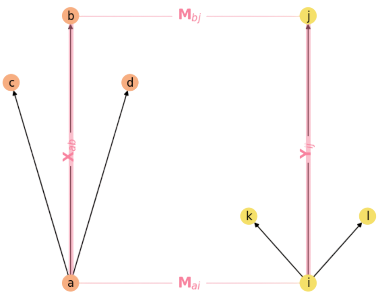
Fig. 2.5 The Rectangle Rule in Graph Matching.#
Quadratic Cost function. A function that counts the number of rectangles given by a matching matrix \(\mathbf{M}\) is simply:
where \(1/2\) factor removes rectangles counted twice (see the explanation to follow).
Consider for instance the graphs \(X\) and \(Y\) in the previous section (see Fig. 2.3). Let us count the number of rectangles por a particular matching using the matricial formulation and the above function.
Firstly, we have the adjacency matrices
The matching matrix for the assignment in Fig. 2.4 is given by
Let us fix the matricial version of \(F(\mathbf{M})\).
Mapping. We commence by analyzing the product \(\mathbf{X}\mathbf{M}\) which maps the nodes in \(X\) to those in \(Y\) via the matching matrix \(\mathbf{M}\):
In our example:
Each column of \(\mathbf{M}\) has at most one \(1\), we have:
where \(b^{\ast}\in {\cal N}_a\) is the neighbor of \(a\) that matches \(i\), if any. Therefore:
where \({\cal M}\) is the matching graph (includes links of \(X\), \(Y\) and \(M\) as in Fig. 2.4).
Therefore, \(\mathbf{X}\mathbf{M}\) has the following paths in \({\cal M}\) (one per each \(1\) in the matrix):
For instance, we show the above paths in Fig. 2.6 and Fig. 2.7.
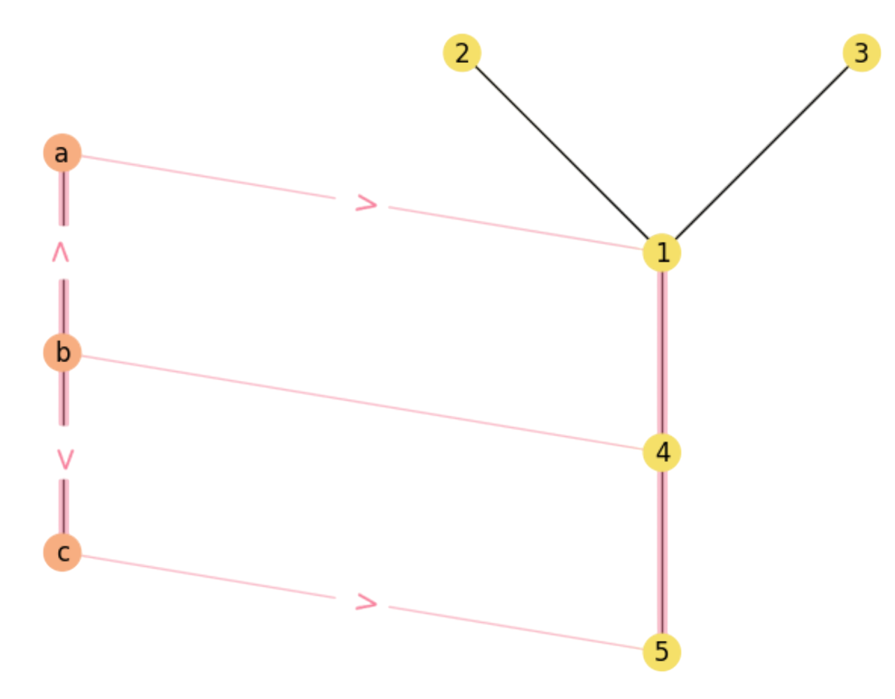
Fig. 2.6 Matching paths \(b\rightarrow a\rightarrow 1\) and \(b\rightarrow c\rightarrow 5\).#
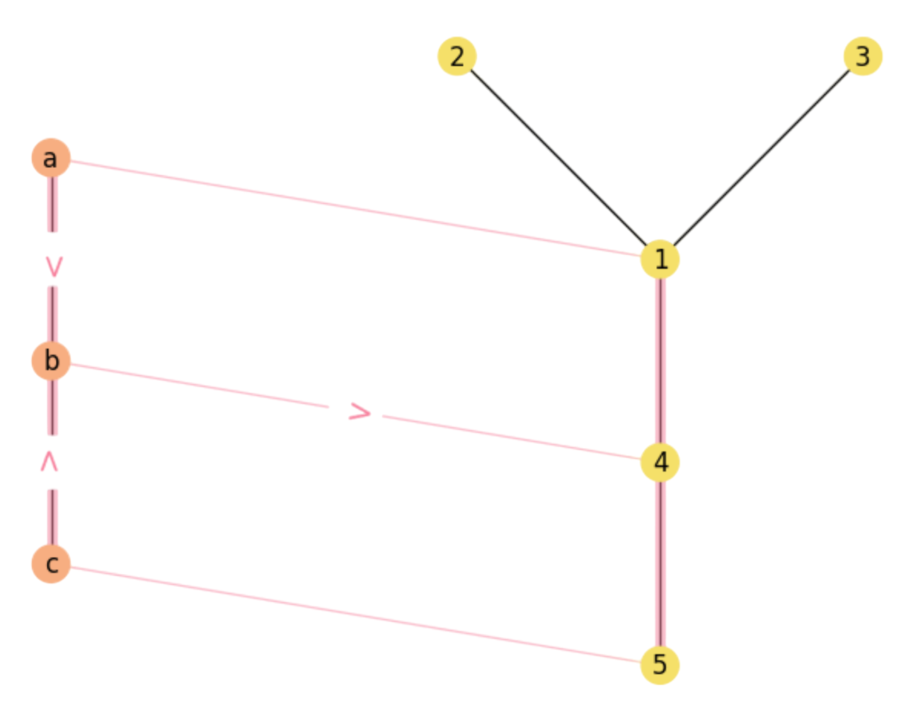
Fig. 2.7 Matching paths \(a\rightarrow b\rightarrow 4\) and \(c\rightarrow b\rightarrow 4\).#
Paths. We continue by analyzing the product \((\mathbf{X}\mathbf{M})\mathbf{Y}\). Intuition: since \(\mathbf{X}\mathbf{M}\) provides paths in \({\cal M}\) between adjacent nodes in \(X\) and then crosses through the matching \(\mathbf{M}\) reaching nodes in \(Y\), the product \((\mathbf{X}\mathbf{M})\mathbf{Y}\) just continues these paths: some of them will end in \(Y\) defining \(3/4\) sides of a rectangle (see below) and some others just travel through \(Y\) without defining any rectangle.
In our example:
Then, the following paths do form \(3/4\) of a rectangle (in bold in \((\mathbf{X}\mathbf{M})\mathbf{Y}\)):
where it is significant the \(2\) paths of \(((\mathbf{X}\mathbf{M})\mathbf{Y})_{b4}\) between nodes \(b\in V\) and \(4\in V'\) (see Fig. 2.8):
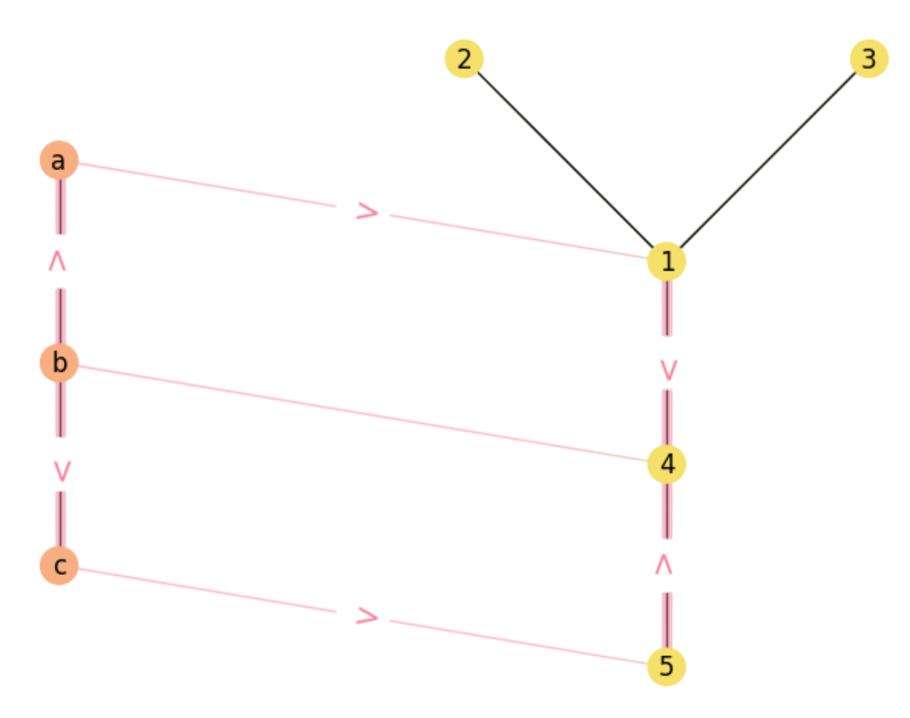
Fig. 2.8 Two \(3/4\) matching paths \(b\rightarrow a\rightarrow 1\rightarrow 4\) and \(b\rightarrow c\rightarrow 5\rightarrow 4\).#
On the other hand, theses other paths do not form \(3/4\) of a rectangle:
For instance, paths \(a\gg b\rightarrow 4\gg 5\) and \(c\gg b\rightarrow 4\gg 1\) diverge from rectangles where the notation \(\gg\) denotes the first and last edges of the paths (see Fig. 2.9).
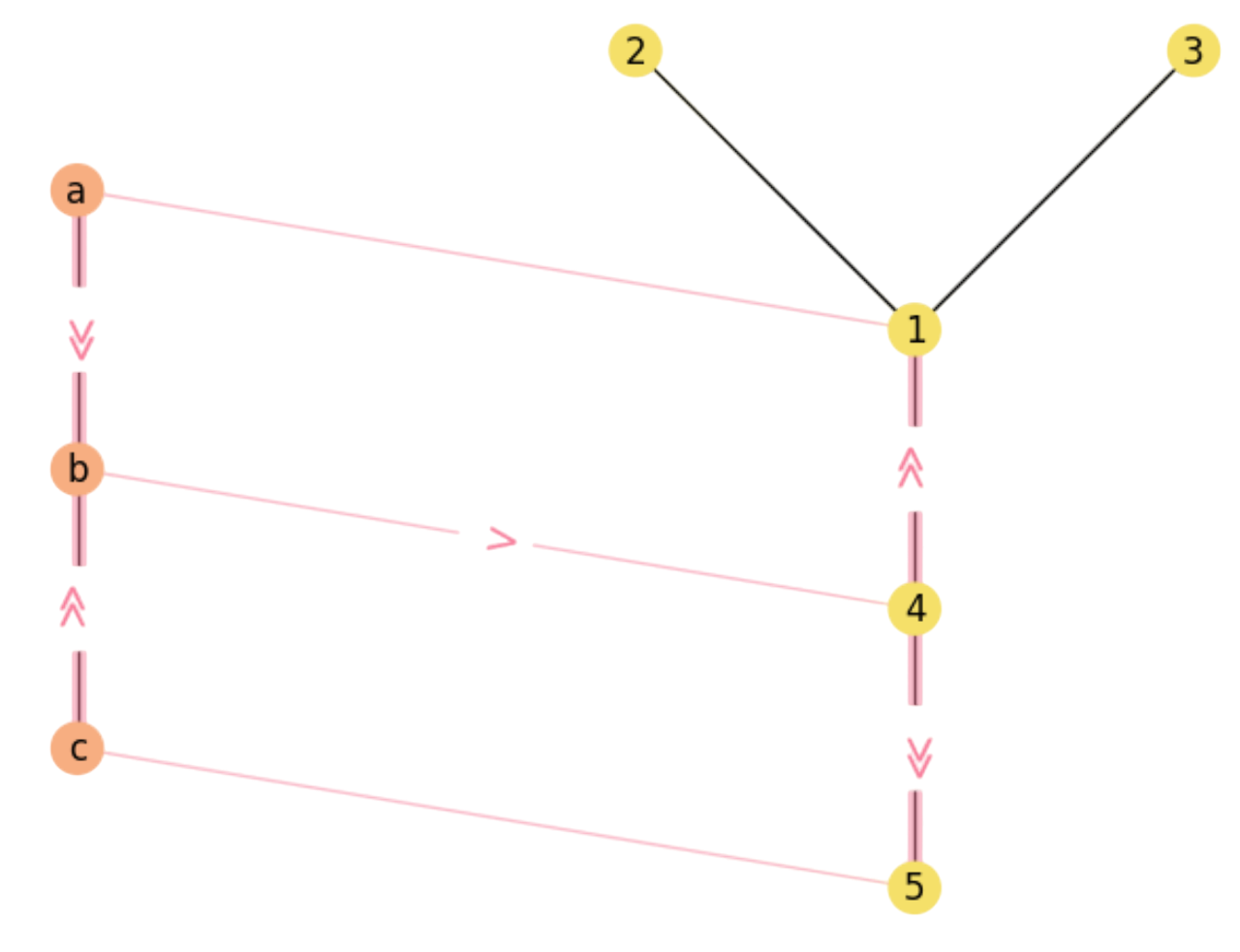
Fig. 2.9 Paths \(a\gg b\rightarrow 4\gg 5\) and \(c\gg b\rightarrow 4\gg 1\) diverge from rectangles.#
Similarly, paths \(b\gg a\rightarrow 1\gg 2\) and \(b\gg a\rightarrow 1\gg 3\) diverge even more clearly from ending up in rectangles (see Fig. 2.10).
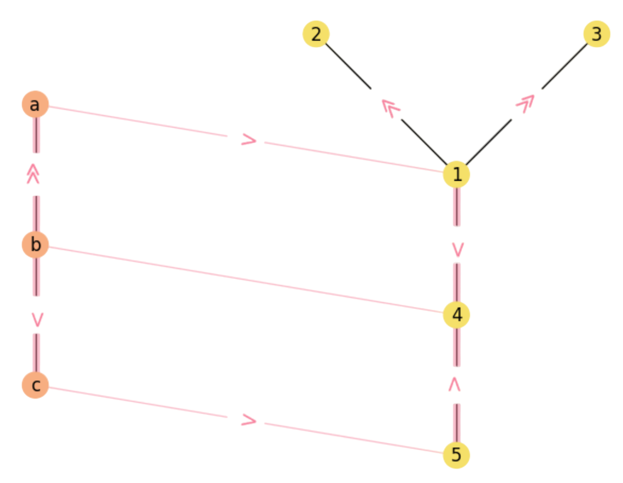
Fig. 2.10 Remaining diverging paths in \({\cal M}\).#
Closing rectangles. Once we have \((\mathbf{X}\mathbf{M})\mathbf{Y}\) we simply perform a pointwise multiplication (Hadamard product) to close the rectangle:
In our example:
Note that \(a\) closes \(1\) rectangle, \(c\) closes \(1\) and \(b\) closes \(2\) (one for \(a\) and another one for \(c\)). Therefore the multiplication \(((\mathbf{X}\mathbf{M})\mathbf{Y})\odot \mathbf{M}\) simply filters out impossible rectangles. The result is in Fig. 2.11.
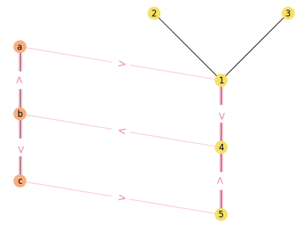
Fig. 2.11 Final rectangles in \({\cal M}\).#
Counting. Note that the number of rectangles comes naturally from
which is \(2\) in this case, as expected! Let us review these concepts in the following exercise:
Exercise. Given the following graphs \(X\) and \(Y\):
\(
\begin{aligned}
&\begin{array}{cll}
\text{Graph} & \text{Nodes} & \text{Edges}\\
X & V=\{a,b,c\} & E=\{(a,b),(b,c)\}\\
Y & V'=\{1,2,3,4,5\} & E=\{(1,2),(1,3),(2,4),(3,4),(1,5),(2,5)\}\\
\end{array}
\end{aligned}
\)
a) Draw them so that the assignment \(f=[(a,1),(b,2),(c,3)]\) is clearly visisble. Is \(X\) a subgraph of \(Y\)? If so, what is the maximal number of rectangles to close in \({\cal M}(f^{\ast})\) and find an optimal assignment \(f^{\ast}\).
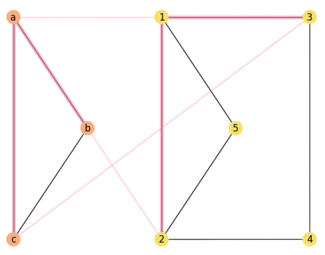
Fig. 2.12 Matching graph \({\cal M}\) for \(f=[(a,1),(b,2),(c,3)]\).#
In Fig. 2.12, we show a 3D projection of both graphs where the assignment is clearly visible. Clearly, \(X\) is a subgraph of \(Y\). As a result, we can map all vertices and edges of \(X\) to \(Y\), closing at most \(3\) rectangles.
b) Is that optimal assignment unique? Compute the maximum number of rectangles by matricially evaluating \(M^{\ast}\), the matching matrix corresponding to an optimal assignment. Indicate the matching paths in each step.
In this case the optimal assignment is unique: it comes from matching the notable vertices between both graphs and it is \(f=[(a,1),(b,2),(c,5)]\) since this is the only way to embed \(X\) in \(Y\) completely (see Fig. 2.13).
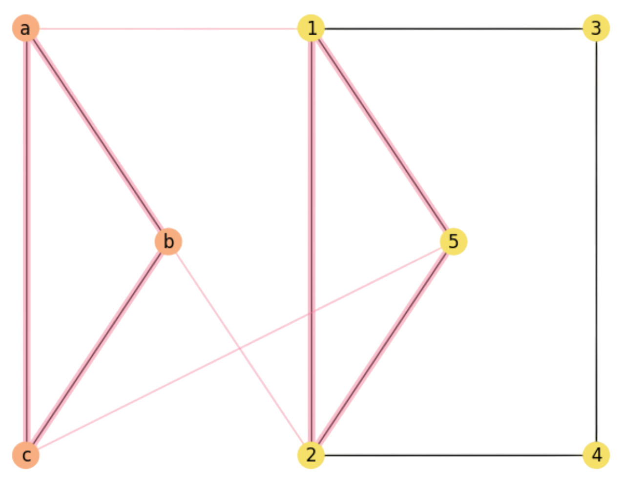
Fig. 2.13 Matching graph \({\cal M}\) for \(f=[(a,1),(b,2),(c,5)]\).#
Matricially, we have
\(
\begin{align}
\mathbf{X} =
\begin{array}{l}
a\\
b\\
c\\
\end{array}
\begin{bmatrix}
0 & 1 & 1 \\
1 & 0 & 1 \\
1 & 1 & 0 \\
\end{bmatrix}
\;\;
\mathbf{Y} =
\begin{array}{l}
1\\
2\\
3\\
4\\
5\\
\end{array}
\begin{bmatrix}
0 & 1 & 1 & 0 & 1\\
1 & 0 & 0 & 1 & 1\\
1 & 0 & 0 & 1 & 0\\
0 & 1 & 1 & 0 & 0\\
1 & 1 & 0 & 0 & 0\\
\end{bmatrix}
\;\;\text{and}\;\;
\mathbf{M}^{\ast} = \begin{array}{l}
a\\
b\\
c\\
\end{array}
\begin{bmatrix}
1 & 0 & 0 & 0 & 0 \\
0 & 1 & 0 & 0 & 0 \\
0 & 0 & 0 & 0 & 1 \\
\end{bmatrix}
\end{align}
\)
Then, we proceed to evaluate
\(
F(\mathbf{M}^{\ast}) = \frac{1}{2}\sum_{a}\sum_{i}(((\mathbf{X}\mathbf{M}^{\ast})\mathbf{Y})\odot \mathbf{M}^{\ast})_{ai}\;,
\)
Step 1: Compute \(\mathbf{X}\mathbf{M}^{\ast}\):
\(
\begin{align}
\mathbf{X}\mathbf{M}^{\ast} =
\begin{array}{l}
a\\
b\\
c\\
\end{array}
\begin{bmatrix}
0 & 1 & 1 \\
1 & 0 & 1 \\
1 & 1 & 0 \\
\end{bmatrix}
\;\cdot \;
\begin{array}{l}
a\\
b\\
c\\
\end{array}
\begin{bmatrix}
1 & 0 & 0 & 0 & 0 \\
0 & 1 & 0 & 0 & 0 \\
0 & 0 & 0 & 0 & 1 \\
\end{bmatrix} =
\begin{bmatrix}
0 & 1 & 0 & 0 & 1\\
1 & 0 & 0 & 0 & 1\\
1 & 1 & 0 & 0 & 0\\
\end{bmatrix}
\end{align}
\)
And the paths so far are:
\(
\begin{align}
(\mathbf{X}\mathbf{M}^{\ast})_{a2} &= a\rightarrow b\rightarrow 2\\
(\mathbf{X}\mathbf{M}^{\ast})_{a5} &= a\rightarrow c\rightarrow 5\\
(\mathbf{X}\mathbf{M}^{\ast})_{b1} &= b\rightarrow a\rightarrow 1\\
(\mathbf{X}\mathbf{M}^{\ast})_{b5} &= b\rightarrow c\rightarrow 5\\
(\mathbf{X}\mathbf{M}^{\ast})_{c1} &= c\rightarrow a\rightarrow 1\\
(\mathbf{X}\mathbf{M}^{\ast})_{c2} &= c\rightarrow b\rightarrow 2\\
\end{align}
\)
Step 2: Compute \((\mathbf{X}\mathbf{M}^{\ast})\mathbf{Y}\):
\(
\begin{align}
(\mathbf{X}\mathbf{M}^{\ast})\mathbf{Y} =
\begin{array}{l}
a\\
b\\
c\\
\end{array}
\begin{bmatrix}
0 & 1 & 0 & 0 & 1\\
1 & 0 & 0 & 0 & 1\\
1 & 1 & 0 & 0 & 0\\
\end{bmatrix}
\cdot\;
\begin{array}{l}
1\\
2\\
3\\
4\\
5\\
\end{array}
\begin{bmatrix}
0 & 1 & 1 & 0 & 1\\
1 & 0 & 0 & 1 & 1\\
1 & 0 & 0 & 1 & 0\\
0 & 1 & 1 & 0 & 0\\
1 & 1 & 0 & 0 & 0\\
\end{bmatrix} =
\begin{bmatrix}
2 & 1 & 0 & 1 & 1\\
1 & 2 & 1 & 0 & 1\\
1 & 1 & 1 & 1 & 2\\
\end{bmatrix}
\end{align}
\)
And the \(3/4\)-rectangle paths are:
\(
\begin{align}
((\mathbf{X}\mathbf{M}^{\ast})\mathbf{Y})_{a1} &= a\rightarrow b\rightarrow 2\rightarrow 1 + a\rightarrow c\rightarrow 5\rightarrow 1\\
((\mathbf{X}\mathbf{M}^{\ast})\mathbf{Y})_{a2} &= a\rightarrow c\rightarrow 5\rightarrow 2\\
((\mathbf{X}\mathbf{M}^{\ast})\mathbf{Y})_{a4} &= a\rightarrow b\rightarrow 2\rightarrow 4\\
((\mathbf{X}\mathbf{M}^{\ast})\mathbf{Y})_{a5} &= a\rightarrow b\rightarrow 2\rightarrow 5\\
((\mathbf{X}\mathbf{M}^{\ast})\mathbf{Y})_{b1} &= b\rightarrow c\rightarrow 5\rightarrow 1\\
((\mathbf{X}\mathbf{M}^{\ast})\mathbf{Y})_{b2} &= b\rightarrow a\rightarrow 1\rightarrow 2 +
b\rightarrow c\rightarrow 5\rightarrow 2\\
((\mathbf{X}\mathbf{M}^{\ast})\mathbf{Y})_{b3} &= b\rightarrow a\rightarrow 1\rightarrow 3\\
((\mathbf{X}\mathbf{M}^{\ast})\mathbf{Y})_{b5} &= b\rightarrow a\rightarrow 1\rightarrow 5\\
((\mathbf{X}\mathbf{M}^{\ast})\mathbf{Y})_{c1} &= c\rightarrow b\rightarrow 2\rightarrow 1\\
((\mathbf{X}\mathbf{M}^{\ast})\mathbf{Y})_{c2} &= c\rightarrow a\rightarrow 1\rightarrow 2\\
((\mathbf{X}\mathbf{M}^{\ast})\mathbf{Y})_{c3} &= c\rightarrow a\rightarrow 1\rightarrow 3\\
((\mathbf{X}\mathbf{M}^{\ast})\mathbf{Y})_{c4} &= c\rightarrow b\rightarrow 2\rightarrow 4\\
((\mathbf{X}\mathbf{M}^{\ast})\mathbf{Y})_{c5} &= c\rightarrow a\rightarrow 1\rightarrow 5 +
c\rightarrow b\rightarrow 2\rightarrow 5\\
\end{align}
\)
Step 3. We higlight the correct matches and apply Hadamard product:
\(
\begin{align}
((\mathbf{X}\mathbf{M}^{\ast})\mathbf{Y})\odot \mathbf{M}^{\ast} =
\begin{bmatrix}
\mathbf{2} & 1 & 0 & 1 & 1\\
1 & \mathbf{2} & 1 & 0 & 1\\
1 & 1 & 1 & 1 & \mathbf{2}\\
\end{bmatrix}
\odot\;
\begin{bmatrix}
1 & 0 & 0 & 0 & 0 \\
0 & 1 & 0 & 0 & 0 \\
0 & 0 & 0 & 0 & 1 \\
\end{bmatrix}
\end{align}
\)
Finally, if we sum all the components of the Hadamard product and divide by \(2\) we have \(3\) rectangles as shown in Fig. 2.13. We are done!
2.2.3. Integer Constraints: QAP#
We have clarified an objective function of MCS (graph matching) \(F(\mathbf{M})\) interpretation for a particular \(\mathbf{M}\in\{0,1\}^{n\times m}\) (number of rectangles). The function is quadratic in \(\mathbf{M}\) since it requires two multiplications of the matching matrix for its evaluation, but evaluating it takes \(O(n^4)\).
In addition, the structure of \(\mathbf{M}\) is not simply binary. Since each candidate assignment \(f\) encoded by this matrix must be an injective (one-to-one) function \(f:V\rightarrow V'\) we have that for \(m\le n\):
i.e. each row/column cannot have more than one \(1\). Some precisions:
Formally, all row/column may be all-zeros but if they are, then we do not have a solution.
In particular, we need to match a coumple of vertices to close a single rectangle. Therefore we need at least to columns with a single one placed in different rows.
Thus, the above notation means that if one row/column is all-zeros there is only one of them which is not!
Ideally, for \(m\le n\) we should have \(m\) columns with a \(1\) all placed in different rows.
This constrained nature of the so called Quadratic Assignment Problem (QAP) is what makes it NP:
Therefore, the QAP (we use this name in the following) is originally posed in terms of Integer Programming (IP) since the unknowns to discover are binary \(m\times n\) matrices \(\mathbf{M}\in\{0,1\}^{m\times n}\) subject to be in \({\cal P}\).
In particular, if \(m=n\) (both graphs have the same number of nodes), then:
\({\cal P}\) becomes \(\Pi_n\), the space of permutations of order \(n\) and we have \(n!\) bijections \(f=\pi:V\rightarrow V'\).
Each matrix \(\mathbf{M}\) encodes a permutation \(\pi(a),\pi(b),\ldots\), where \(V=\{a,b,\ldots\}\) with \(|V|=n\) are the rows of \(\mathbf{M}\) (each one with a unique \(1\) at different columns.
Then \(V'=\{\pi(i):i\in\{a,b,c,\ldots\}\}\) with \(|V'|=n\) and \(\pi^{-1}(i)\in V\) does exist and it is unique.
More formally:
where we have transformed the inequality constraints into equality ones!
The Permutohedron is a useful means of visualizing the space of solutions \(\Pi_n\). Each point is a permutation \(\pi\) and it has \(n-1\) neighbors. Given \(\pi\), its neighboring permutations \(\pi'\in {\cal N}_{\pi}\) differ from \(\pi\) in one transposition, i.e. one interchange between two components.
For instance, in Fig. 2.14 we show \(\Pi_4\). It has \(n!=24\) nodes with \(n-1=3\) neighbors each. For instance, the neighbors of \(\pi=[3,4,2,1]\) are \({\cal N}_{\pi}=\{[2,4,3,1],[3,4,1,2],[4,3,2,1]\}\), where \(\pi'=[2,4,3,1]\) is the result of interchanging (transposing) \(2\) and \(3\) in \(\pi=[3,4,2,1]\).
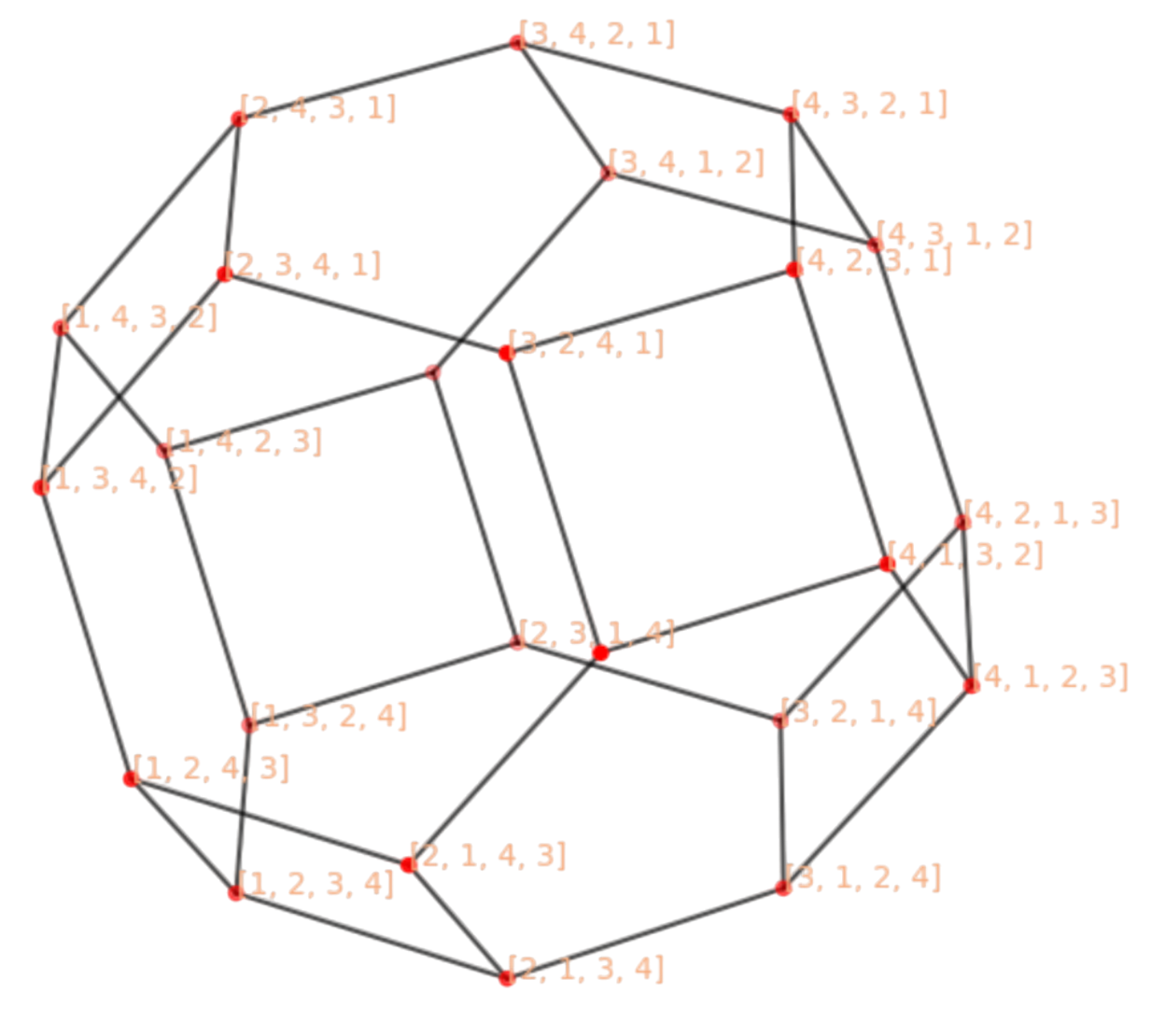
Fig. 2.14 Permutohedron for of order \(n=4\). Please define the unlabeled nodes.#
2.3. Simulated Annealing#
The Permutohedron provides a glimpse of the discrete seach space, specially because it highlighs its topology, i.e. its local structure.
With this instrument to hand, it is natural to envision intelligent search as a random walk between an initial permutation \(\pi^0\) and a final one \(\pi^{\ast}\):
The intelligence is partially provided by the objective function \(F(\pi)\) that discriminates between good and bad solutions.
The search strategy is what exploits the knowledge provided by the objective function. One of the simplest strategies is that of a random walk (RW) \(\pi^0\rightarrow\pi^1\rightarrow\ldots\rightarrow \pi^{\ast}\) inside \(\Pi_n\).
Simulated Annealing (SA) is a principled way of combining intelligence and RW-search. It works as follows:
Let \(\Omega\) be the search space and \(\omega\in \Omega\) a discrete state, then we define a Markov chain \(X_0,X_1,\ldots\) for a maximization problem as follows:
where \(\Delta F:=F(\omega')-F(\omega)\) and \(\beta(t):=\frac{1}{T(t)}\) where \(T\) is the computational temperature. Some explanations:
Since we are maximizing \(F\), having \(\Delta F:=F(\omega')-F(\omega)\ge 0\) for \(\omega'\in {\cal N}_{\omega}\) means that \(F(\omega')\ge F(\omega)\), i.e. that we are in the correct way (or at least not in the wrong way!). In this case, we should accept (with probability \(1\)) \(\omega'\) as the new state of the search.
If \(F(\omega')< F(\omega)\), a greedy method or a branch-and-bound should reject \(\omega'\) as a promising direction. However, SA gives a chance of acceptance which is proportional to how far is \(\omega'\) of being promising, which is \(\Delta F = F(\omega')-F(\omega)< 0\).
However, if \(F(\omega')< F(\omega)\), the chance of accepting \(\omega'\) must depend of the stage of the search process where we take the decision. This stage is parameterized by the computational temperature \(\beta(t)=\frac{1}{T(t)}\)
Suppose that the computational temperature is \(T(t)\) is a monotonic decreasing function with \(t\) such as \(T(t)=\frac{1}{\log(1+t)}\). This is why this is called an annealing schedule Then:
At \(t\rightarrow 0\) (early stages of the search) the chance should be hight. Then, we usually set \(T(0)\rightarrow\infty\) (high temperature). As \(\Delta F<0\), then \(\exp(\beta(t)\cdot \Delta F)\) does not decays too much, since it is attenuated. As a result, solutions \(\omega'\) with \(\Delta F<0\) are typically accepted if \(|\Delta F<0|\) is small enough. The larger \(|\Delta F<0|\) the more probable that \(\omega'\) is consider an extremal event (part of the queue of the exponential) and thus discarded.
However, for \(t\rightarrow \infty\), we have \(T(t)\rightarrow 0\) (low temperature). The same decrement \(|\Delta F<0|\) that was admissible for smaller values of \(t\) is not yet accepted because SA behaves like a greedy method.
Algorithm 2.1 (Metropolis-Hastings)
Inputs Given a function \(F(\omega)\), an annealing schedule \(T(t)\) and an inital state \(\omega_0\)
Output \(\omega^{\ast}=\arg\max_{\omega\in\Omega} F(\omega)\)
convegence = False
\(\omega_{old}\leftarrow \omega_0\)
\(t\leftarrow 0\)
while \(\neg\) convergence:
Select \(\omega'\in {\cal N}_{\omega}\)
Calculate \(\Delta F=F(\omega')-F(\omega_{old})\)
if \(\Delta F\ge 0\) then \(\omega_{new}\leftarrow \omega'\)
else:
Draw \(p\in [0,1]\)
\(q\leftarrow \exp\left(\frac{\Delta F}{T(t)}\right)\)
if \(q\ge p\) then \(\omega_{new}\leftarrow \omega'\)
\(t\leftarrow t+1\)
\(T(t)\leftarrow \frac{1}{\log(1 + t)}\)
convergence = \((T(t)<T_{min})\) or \((t>t_{max})\)
return \(\omega_{new}\)
2.3.1. Approximating QAP with SA#
Let us apply SA to approximate the QAP. To that end, we are going to match the Aspirin’s structure (see Fig. 2.16-Left) with a random permutation of its vertices (Fig. 2.16-Right). The left graph with nodes \(V=\{a,b,\ldots,m\}\) and links, mimics the structure of the Aspirin. In this first approach we discard, for the moment, both nodes (atom) labels (\(\text{C}\),\(\text{O}\) and \(\text{OH}\)) and edges (bonds) labels (single, double).
On the right, the graph has nodes \(V'=\{1,2,\ldots,13\}\). Since \(|V|=|V'|=13\), there state space \(\Omega\) is given by the \(\Pi_{n=13}\) Permutohedron, with \(n!\approx 6\times 10^{9}\) states, each one with \(n-1=12\) edges.
We know that the optimal permutation \(\pi^{\ast}\) is given by \(\pi^{\ast}(a)=1,\pi^{\ast}(b)=2,\ldots, \pi^{\ast}(m)=13\), i.e. \(\mathbf{M}^{\ast}=\mathbf{I}_n\) is the identity matrix of dimension \(n\). However, we assume a realistic case where the input permutation \(\pi^0\) is rather different from the optimal one:
1) Initial Matching. However, instead of starting SA with a random \(\pi^0\), it is a good practice to compute a greedy approximation. In the case of graph matching or QAP, a greedy algorithm may rely on matching \(a,b,c,\ldots\) with nodes \(1,2,3,\ldots\) in such a way that it is preferred to match nodes with the largest number of neighbors (degree) as possible.
Then, the greedy matching leads to
We check Fig. 2.16, where we plot the final approximation of SA with \(10\) closing rectangles, that the greedy \(\pi^0\) is consistent with matching nodes with mutually largerst degrees:
We underlined the matchings with largest degrees (maximum degree is \(3\)): \(c\rightarrow 5\), \(e\rightarrow 1\).
One of the risks of greedy matching is that we may be stuck in a local maximum, which really happens (SA here recovers from \(e\rightarrow 1\) but not from \(c\rightarrow 5\)).
However, the proper annealing scheduling typically takes the search out of local optima in the early stages of the search.
2) Neighboring. The second aspect to define when applying SA to the QAP is how to ensure proper neighborhoods \({\cal N}_{\omega}\). In other words, if given \(\omega\) we choose as \(\omega'\) an arbitrarily large random variation, we may miss the irreducibility property of the Markov chain (all states must be reached).
Then, a good way of navigating properly through the search space (the Permutohedron \(\Pi_n\) in this case) is to:
Choose randomly if we are going to interchange rows or colums in \(\mathbf{M}_{\omega}\).
Interchange two rows (or columns) whose indexes are randomly chosen. The result is \(\mathbf{M}_{\omega'}\)
This is equivalent to perform a transposition in the Permutohedron \(\Pi_n\).
3)Annealing Schedule. The last ingredient to set is a proper temperature cooling (annealing schedule) and the specific values \(T_0\) and \(T_f\).
In this example, we simply make \(T(t+1)=T(t)-\alpha\cdot T(t)=(1-\alpha)\cdot T(t)\) with \(\alpha\ll 1\).
This leads to a neg-exponential decrease since:
This succession is decreasing since we only multiply \(T(0)\) by a decreasing fraction. Actually, we have set \(T(0)=1/5=0.2\) and \(\alpha = 1/1.075\approx 0.93\). The exponential decrease can be seen by looking at the logarithmic transformation (exponentials are lines in log space):
Since \((1-\alpha)<1\) then its log is negative!
This schedule is a bit agressive but playing a bit with \(\alpha\) we can close \(10-11\) rectangles from \(13\) possible (this is the mumber of edges of the Aspirin graph).
In Fig. 2.15 we play with different values of \(\alpha\). For the sake of clarity, herein we only represent the best cost obtained so far. Note that for different regimes we get different results, in this case between \(0\) and \(11\) rectangles. It is interesting to note that:
The best result is obtained with one of the smallest \(\alpha\)s (\(\alpha=0.85\))
The annealing schedules tend to increase more the objective function \(F\) in the early stages of the seach where SA is more free to explore!
Note that the most strict schedule (\(\alpha=0.93\)) reaches \(9\) rectangles in the middle stages and finaly peaks \(10\) rectangles. This is the solution showed in Fig. 2.16.
The right image shows the negligible differences betweeen the annealing schedules in the log-log domain.
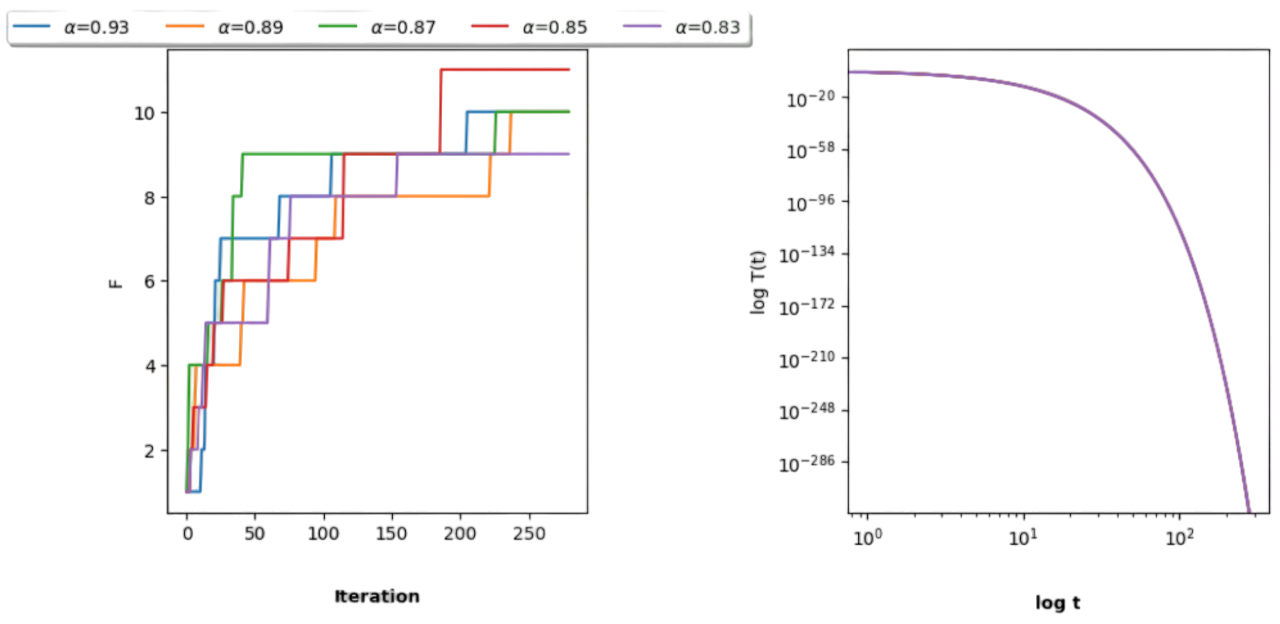
Fig. 2.15 Playing with \(\alpha\) for different annealing schedules.#
4)Understanding the solution. Last, but by no means least, we have to interpret to what extent our \(F\) reaches or not an interesting solution. Herein, interesting means global. For instance:
The solution in Fig. 2.16 captures mainly the central hexagon, although under a rotation around the \(g-i\) axis and a flipping or torsion wrt the vertical: edge \(f-e\) becomes \(8-10\), but edge \(h-i\) becomes \(3-9\).
The top part of the molecule in the Left matches a bottom part of that of the Right, indicating a global deformation.
Also the bottom-left part of the molecule in the Left matches the top part of that in the Right (again a deformation).
Overall, the largest subgraphs are correctly matched but the smallest ones are misplaced.
Therefore, althoug the solution obtained seems quantitatively global it is partially qualitatively global. This reveals a need of making the objective function more informative (we will come back to this point later on).
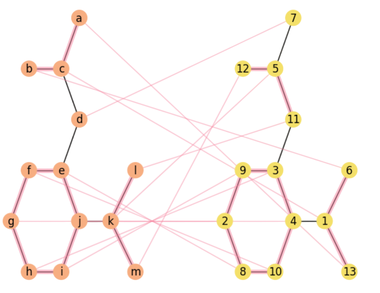
Fig. 2.16 Approximating the Aspirin’s Isomorphism with SA.#
2.3.2. Interpretation of SA#
Intuitive interpretation. From an intuitive point of view, SA can be described as follows Hoffmann and Buhmann 1997:
Cost differences between neighboring states act as a force field.
The effect of the computational temperature can be interpreted as a random force with an amplitude proportional to T.
Valleys and peaks with a cost difference less than T are smeared out and vanish in the stochastic search. Vanishing is more likely to happen in the early stages of the search where we need to scape from local (subobtimal) solutions.
Methodological Interpretation. In the AI jargon, \(F\) is considered an heuristic and SA is considered a meta-heuristic:
Heuristic. This term was introduced by Herbert Simon and it loosely means “seach shortcut”, i.e. some mechanism for deciding what solution is interesting and what is not in a potentially large space of solutions. This concept is our subject. Herein, it is the number of rectangles.
Meta-Heuristic are procedures that “modulate the application of a heuristic”. SA is a metaheuristic because it decides when the search is more stochastic and when it becomes more greedy.
Formal interpretation. Remember that the Metropolis Algorithm implements an irreducible Markov chain \(X_0,X_1,\ldots,X_t\) along \(\Omega\). This Markov chain is stationary i.e. it converges to a given probability distribution \(G\) which means that after a given time step \(t\) if \(X_{t}\sim G(\omega)\) then also \(X_{t+1}\sim G(\omega)\). The stationary distribution is
independently of the choose of \(X_0\). In this case, the stationary distribution \(G(\omega)\) is
which is known as the Gibbs distribution. Look, for instance, at the \(q\) variable at the step \(4.2.\) of the Metropolis-Hastings algorithm:
Therefore, the so-called acceptance probability is a ratio between two “Gibbsian” probabilities!. Note that in the Gibbs distribution, for a given \(\beta\) the states \(\omega\in \Omega\) with larger \(F(\omega)\) are more probable. As a result, \(q\) is the largest possible when \(F(\omega')\gg F(\omega_{old})\) (of course for this \(\beta\)).
Consequently, SA can be seen as a sampling process that converges to the global optimal \(\omega^{\ast}\) of \(F(\omega)\) if the annealing schedule is a proper one. However, what is the fomal role of the temperature (or its inverse: \(\beta\))? Solving this question is a good excuse to dive into Information Theory, a mathematical discipline which is built on top of Probability and it is fundamental to undestanding intelligent search.
2.3.3. Gibbs Sampling#
SA shows that intelligent search can be seen as deploying random walks for exploring combinatorial spaces such as \(\Pi_n\). For this section, we need a key probabilistic concept: the expectation of a random variable.
Remember that the expectation of a discrete random variable \(\omega\) is defined as follows:
Expectation gives us an idea of the spatial concentration of the values \(\omega\in\Omega\) attending to \(p(X=\omega)\). Actually \(E(X)\) can be seen as the most representative of this values (i.e. the most likely of them).
For determining \(E(X)\) it is mandatory to know all the probabilities \(p(X=\omega)\).
However, what if \(p(X=\omega)=G(X)\), i.e. if \(X\) is Gibbsian?. This is the case of \(X=F(\omega)\), the value of the cost function. In this latter case,
is the expected cost. Can we really calculate it? Well, it is impossible to do it analitically because:
We should know all the values \(F(\omega)\). This is equivalent to solve the problem encoded by this cost function by means of brute force. Remember that for the QAP this implies to evaluate all the states of the Permutohedron, i.e. \(n!\) states whose individual evaluation takes \(O(n^4)\).
The Gibbs distribution seems to be restricted to a given \(\beta\). We should evaluate \(Z=\sum_{\omega\in\Omega}G(\omega)\), a very large sum, for that particular \(\beta\). Therefore, \(E(X)\) seems to be \(\beta-\)dependent as well.
Instead, the Metropolis-Hastings algorithm allows us to approximate \(E(X)\) as follows:
where \(\omega_1,\omega_2,\ldots, \omega_r\) are the states visited by the algorithm when it follows an admisible anneling schedule such as \(T(t)=\frac{C}{\log(1+t)}\) where \(C\) is a constant. This means that \(\omega_r\) is accepted at \(T(r)\).
Some related considerations:
The sequence \(\omega_1,\omega_2,\ldots,\) is a random walk along \(\Omega\) which is driven by \(F(\omega)\) and converges to the Gibbs probability.
The lower the temperature \(T(t)\) the closer we become to the Gibbs distribution. Therefore the computational temperature works as a Lagrange parameter to enforce the convergence towards the Gibbs distribution.
Formally, not all the samples \(\omega_1,\omega_2,\ldots,\omega_r\) are generated by \(G(\omega)\) since every random walk has a transient period (unstable values) and we do not know exactly at what time instant we have the convergence, i.e. \(\omega_t\) become proper samples of \(G(\omega)\).
Following Understanding Gibbs Sampling, a good strategy is to start different random walks at different \(X_0\)s (initial permutations in QAP) and track the samples until we can observe some consensus.
In Fig. 2.17, we show three random walks generated from different \(X_0\)s, for the admisible annealing (inverse log) with \(C=3\). None of them reaches the global optimum in \(R=7,000\) iterations. Actually their approximate expectations \(E(X)\) are respectively \(8.637\), \(8.178\) and \(9.371\) if we remove the first \(1,000\) samples (considered as transient regime), whereas we have \(9.051\), \(8.466\), and \(9.791\) if all the samples are included.
What is interesting here is that it is quite difficult to reach the global optimum since:
There are fewer states with that value in general and most of them are sub-optimal. This is indiated by the fact that \(E(X)\ll \omega^{\ast}\) for \(X=F(\omega)\).
In combinatorial problems such as QAP, the cost function has a discrete number of energy levels and this usually leads to plateaus (regions of constast cost) as cooling progresses. For instance, in Fig. 2.17 random search seems blocked in a sub-optimal state, at least for such number of iterations \(R\).
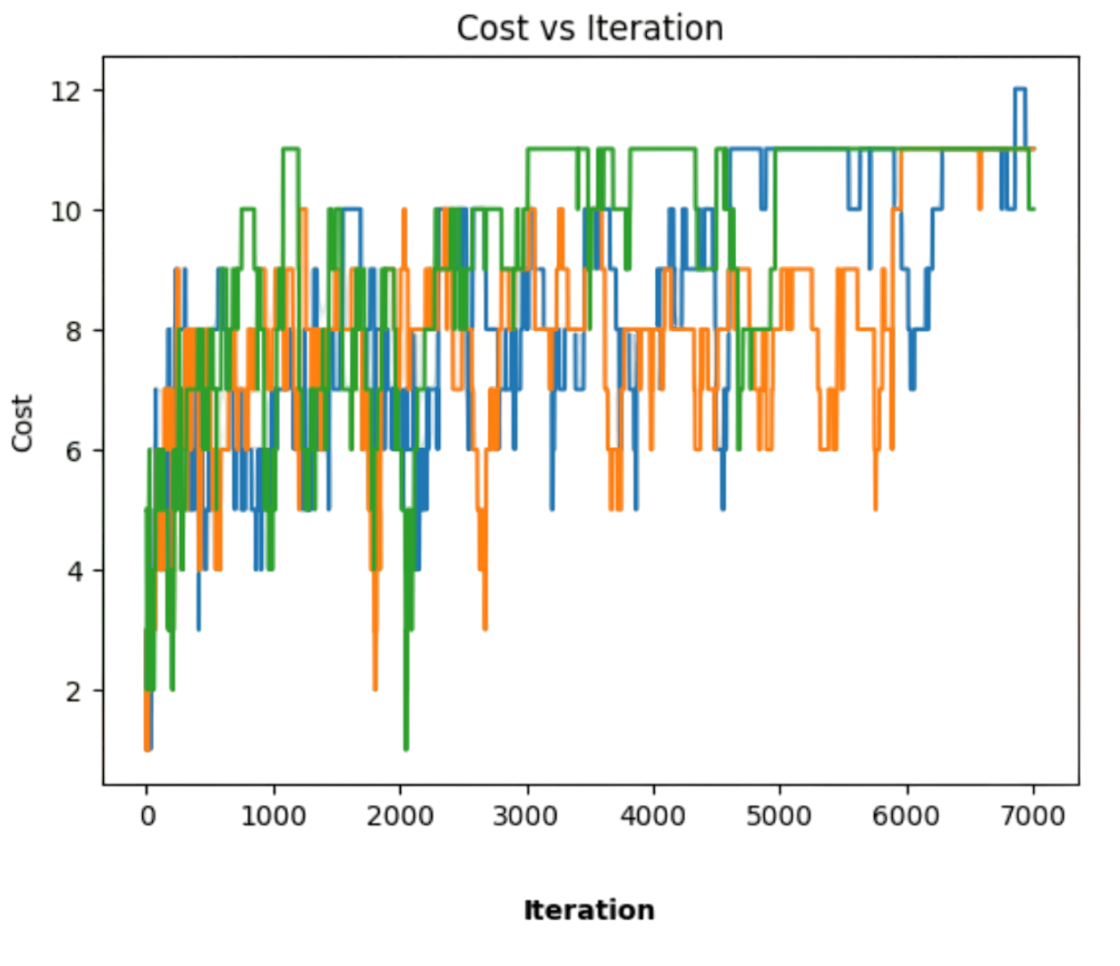
Fig. 2.17 Three random walks along \(\Pi_n\) with differernt \(X_0\)s.#
Note also that herein we have highlighted the main features of SA. Please check the beautiful paper of the Geman’s brothers: Stochastic Relaxation, Gibss Distribution and the Bayesian Restoration of Images one of the most influential papers in all times.
2.3.4. Limitations of SA#
SA is appealing for AI since it allows us to track the global optimum in a sort of random walk. However:
The quality or “intelligence” of the random walk relies on how informative is the cost function. How is information measured? We will address this question later on.
The global optimum is only guaranteed for a slow annealing \(T(t)=\frac{C}{\log(1+t)}\rightarrow 0\). SA has to be slow enough to not missing that global optimum; otherwise SA becomes greedy prematurely. This is an important limitation of SA: remember that for QAP we have to evaluate \(F(\omega)\) at each time \(t\) and it takes \(O(n^4)\).
2.4. Central Clustering#
Deterministic Annealing (DA) emerges as a faster method than SA. In order to motivate this technique it is more convenient to visit another NP problem. This problem is central clustering (or \(k-\)centrer clustering) and it is formulated as follows:
Given a set \({\cal X}=\{\mathbf{x}_1,\mathbf{x_2},\ldots,\mathbf{x}_m\}\subset \mathbb{R}^d\) (\(d-\)dimensional points) and an integer parameter \(k>1\), find a set of \(k\) centers \({\cal C}=\{\mathbf{c}_1,\mathbf{c}_2,\ldots,\mathbf{c}_k\}\subset \mathbb{R}^d\) such that so that the Euclidean distance \(D(\mathbf{x},\mathbf{c})\) of each point \(\mathbf{x}_a\) to its closest center \(\mathbf{c}_i\) is minimal.
2.4.1. Clusters and Prototypes#
A more intuitive formulation is as follows. Let
be a cluster, i.e. a subset of \({\cal X}\) where its elements \(\mathbf{x}_a\) are closer to the cluster’s prototype \(\mathbf{c}_i\) than to any other. Then, the problem is also formulated as follows:
Partition \({\cal X}\) in \(k\) (disjoint) clusters such that the sum of distances between the points and the prototypes is minimal.
Some clarifications:
The problem is a chicken-and-egg problem: a) We need to know the \(k\) centers \(\mathbf{c}_i\) beforehand in order to determine the clusters \(\text{cluster}(\mathbf{c}_i)\) but b) the prototypes have to be determined once the clusters are done according with the criterion of minimal distances.
The NP-hardness of the problem is given by the partitioning flavor. Actually, the worst case complexity is \(O(k^m)\) since each of the \(m\) different points can be exclusively assigned to \(k\) centers (r-permutations with repetition \(P_{\sigma}(m,k)=k^m)\).
The prototypes \(\mathbf{c}_i\) do not necessarily belong to \({\cal X}\) and they must be discovered.
See for instance a well defined problem in Fig. 2.18 where the red dots are ideal centers \(\mathbf{c}_i\) which are the expectations \(\mu_i\) of bidimensional Gaussians \(N(\mu_i,\sigma\mathbf{I})\) with \(\sigma=0.5\).
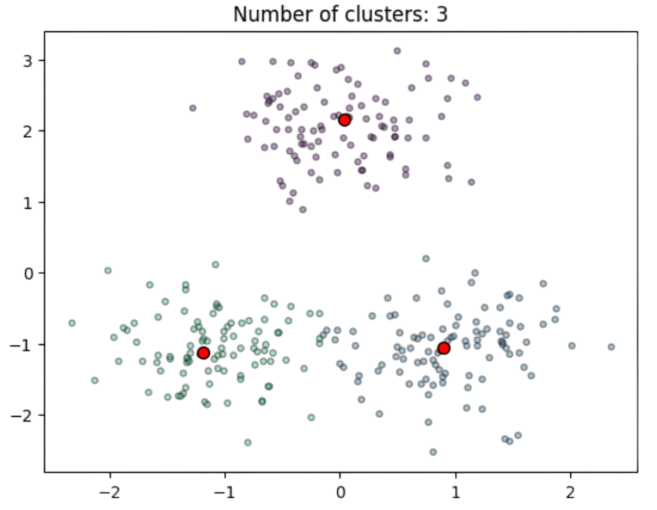
Fig. 2.18 Clusters and estimated prototypes in \(\mathbb{R}^2\).#
2.4.2. Cost Functions#
2.4.2.1. Attractors#
A first compact cost function could be:
where we are interested in \({\cal C}^{\ast}\), the set \(k\) centers/prototypes minimizing the total distance.
In Fig. 2.18, two centers \(\mathbf{c}_1=[-1,-1]^T\) and \(\mathbf{c}_2=[1,-1]^T\) and mutually closer than the third one \(\mathbf{c}_3=[0,2]^T\). Then, if we represent the individual cost of each point \(\mathbf{x}_a\) wrt each center, i.e. \(min_{1\le i\le k}D(\mathbf{x}_a,\mathbf{c}_i)\) (see Fig. 2.19) note that there is well-defined minimum at \(\mathbf{c}_1=[-1,-1]^T\) which we interpret as an attractor or meta-stable state, since it distorts the locations of the other two minima. Note also, that the cost function is clearly non convex and it has many saddle points (see for instance the 3D view in Fig. 2.20)
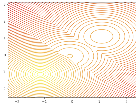
Fig. 2.19 Individual cost wrt closest centers.#
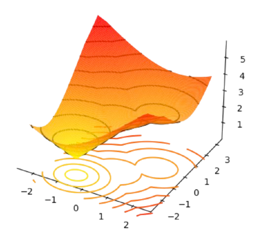
Fig. 2.20 Individual cost wrt closest centers (3D view).#
However, if we also include the point-to-cluster assignment variables \(\mathbf{M}_{ai}\), we aim to jointly minimize:
where each point can be only assigned to a single cluster and all points must be assigned (each row has a single \(1\)).
2.4.2.2. Independence#
Note that the Gibbs distribution for \(F({\cal C},\mathbf{M})\) is
where the negative exponential means that the probability of a solution decays exponentially with the distances beween the points and the cluster centers or prototypes.
Instead of sampling \(\Omega={\cal C}\times{\cal P}\) with SA, where
we are going to assume that the variables \({\cal C}\) and \(\mathbf{M}\) are statitically indepedendent. Then, following the Appendix, we compute the marginal of the Gibbs distribution wrt the assignment matrices:
Now, looking at the sum of neg-exponentials, we observe that the sum is over the legal assignment matrices \(\mathbf{M}\in{\cal P}\) (each point must be assigned to a unique prototype). This means that any legal matrix will be a collection of rows ratisfying:
This means that for each of the \(m\) rows of \(\mathbf{M}\) we have \(k\) options for \(m\) positions, leading to \(k^m\) total legal matrices, i.e. terms in \(\sum_{\mathbf{M}\in {\cal P}}Q(\mathbf{M})\). However, this number can be reduced if we perform a second independence assumption: the assignmnet of a point to a cluster is independent to that of another point (logically this is not true for nearby points but this simplifies the calculations).
This allows us to express the neg-exp sum as the following sum, implementing a logical \(\lor\):
where \(\mathbf{M}^{(1)},\mathbf{M}^{(2)},\ldots,\mathbf{M}^{(m)}\) are the assignment matrices that can be chosen for any particular point \(\mathbf{x}_1,\mathbf{x}_2,\ldots,\mathbf{x}_m\).
Since independence means factorization we have \(\sum\sum\ldots\sum = \sum\cdot\sum\ldots\sum\) as in multiple integration, i.e.:
where the product \(\prod_{a=1}^m\) absorbs the sums \(\sum_{a=1}^m\) inside each exponential.
Now pay attention! This the point where we use the fact that \(\sum_{i=1}^k\mathbf{M}^{(a)}_{ai}=1,\forall a\) (for each row!), i.e. only one cluster will be chosen. Actually, we have an XOR! This leads us to:
Final result. Then, in order to capture the above factorization, the original cost function \(F({\cal C},\mathbf{M})\) must be transformed as follows
which can be computed in \(O(nk)\). Actually, \(F_{\beta} = -\frac{1}{\beta}\log Z\) is usally called the Free Energy.
2.4.2.3. Derivation#
The below DA algorithm for central clustering results from the minimization of the Free energy as follows:
Let us compute the derivative of
wrt each center \(\mathbf{c}_i\):
For \(D(\mathbf{x}_a,\mathbf{c}_i)=||\mathbf{x}_a-\mathbf{c}_i||^2\) we have:
Then, plugging this derivative in the main formula, and expanding the \(Q(\mathbf{x}_a)\), we obtain:
Note that
Then,
Since the optimum is obtained when the gradient is zero, we have:
Therefore, the DA algorithm for central clustering is simply derived from the gradient of the free energy. Summarizing, DA consists in performing gradient descent wrt to each inverse temperature \(\beta\).
2.4.3. Deterministic Annealing#
Deterministic Annealing (DA) is a search technique easily applicable to the central clustering problem (see more details in Keneth Rose’s PhD Thesis).
The basic idea of DA is that for each value of \(\beta=\frac{1}{T}\) we interate two phases for minimizing the free energy \(F_{\beta}({\cal C})\):
Expectation. For fixed centers \(\mathbf{c}_i\), we estimate the probability that any point \(\mathbf{x}_a\) “belongs” to each cluster (“membership”). We denote such probabilities as \(\langle \mathbf{M}_{ai} \rangle\) and they are given by:
Update. For fixed probabilities \(\langle \mathbf{M}_{ai} \rangle\), we update the centers. If \(D(\mathbf{x}_a,\mathbf{c}_i)=||\mathbf{x}_q-\mathbf{c}_i||^2\) (squared Euclidean distance), then we have
i.e. the new (“fuzzy”) centers are the expected centers according to the fixed probabilities or (“memberships”).
Algorithm 2.2 (Deterministic Annealing [Clustering])
Inputs Given a set of points \({\cal X}=\{\mathbf{x}_1,\ldots,\mathbf{x}_m\}\), the free energy \(F_{\beta}({\cal C})\), an annealing schedule \(\beta =1/T(t)\) and an inital state \({\cal C}^0=(\mathbf{c}^0_1,\ldots,\mathbf{c}^0_k)\)
Outputs \({\cal C}^{\ast}=\arg\min_{{\cal C}\in\Omega} F_{\beta\rightarrow\infty}({\cal C})\) and \(\langle \mathbf{M}^{\ast}_{ai}\rangle\)
convegence = False
\(\langle \mathbf{M}^{old}_{ai}\rangle\leftarrow 1\)
\(t\leftarrow 0\)
while \(\neg\) convergence:
for \(\mathbf{x}_a\in {\cal X}\), \(\mathbf{c}_i\in {\cal C}\):
\( \langle \mathbf{M}_{ai} \rangle = \frac{\exp(-\beta D(\mathbf{x}_a,\mathbf{c}_i))}{\sum_{i'=1}^k \exp(-\beta D(\mathbf{x}_a,\mathbf{c}_{i'}))} \)
for \(\mathbf{c}_i\in {\cal C}\):
\( \mathbf{c}_i = \frac{\sum_{a=1}^m \mathbf{x}_a \langle \mathbf{M}_{ai}\rangle}{\sum_{a=1}^m\langle \mathbf{M}_{ai}\rangle} \)
\(t\leftarrow t+1\)
\(T(t)\leftarrow \frac{1}{\log(1 + t)}\)
convergence = \((T(t)<T_{min})\) or \((t>t_{max})\) or \((\sum_{ai}|\langle \mathbf{M}_{ai}\rangle - \langle \mathbf{M}^{old}_{ai}\rangle|\le\epsilon )\)
\(\langle \mathbf{M}^{old}_{ai}\rangle\leftarrow \langle \mathbf{M}_{ai}\rangle\)
return \({\cal C}^{\ast}\), \(\langle M^{\ast}\rangle\)
Some considerations about the above algorithm:
It is deterministic, i.e. we do not draw random numbers at any step of the algoorithm.
The initial (inverse) temperature \(\beta=1/T_{max}\), where \(T_{max}=T(0)\), is used as in SA, to make all the assignments almost equally probable: note that \(e^{-\beta D(\mathbf{x}_a,\mathbf{c}_i)}\rightarrow 1\), if \(\beta\rightarrow 0\). Under these conditions, we have \(\langle M_{ai}\rangle\approx 1/k\).
Initialization. \(T_{max}\) is set to the maximum variance \(\sigma^2_{max}\) of the data. If the data is multidimensional, as it happens usually, \(\sigma^2_{max}\) has an spectral interpretation (PCA).
However, as the algorithm evolves, \(\beta\) increases and the exponential decay becomes more selective: given \(D(\mathbf{x}_a,\mathbf{c}_i)\le D(\mathbf{x}_a,\mathbf{c}_j)+\alpha\), the second distance decays exponentially faster than the first as \(\beta\) increases.
Alternating Expectation and Update. Given the probabilities \(\langle M_{ai}\rangle\) we update the centers \(\mathbf{c}_i\) and then we re-compute the probabilities until a “fixed point” (stable assignment/centers) is reached.
Convervence. The algorithm converges to the nearest local optimum of the free energy to the initialization point \({\cal C}^0\). We add the condition \(\sum_{ai}|\langle \mathbf{M}_{ai}\rangle - \langle \mathbf{M}^{old}_{ai}\rangle|\le\epsilon\) with \(\epsilon>0\), which means that the algorithm stops if the \(\langle \mathbf{M}_{ai}\rangle\) are stable enough. For instance, if we start by setting \(\langle M_{ai}\rangle\approx 1/k\), the algorithm only performs a single iteration. Why? Because the centers in step 4.2. are not modified at all.
Complexity. Each iteration takes \(O(mk)\) and the number of iterations can be accelerated by a faster annealing schedule.
Outputs. The algorithm returns the best centers \({\cal C}^{\ast}\) and the optimal assignments \(\langle \mathbf{M}_{ai}^{\ast}\rangle\) where a point \(\mathbf{x}_a\) is assigned to the cluster centered at \(\mathbf{c}_{i'}\) if:
We show how the algorithm works in one-dimensional points in the following exercise:
Exercise. Given the following points \({\cal X}=\{1,2,3,7,7.5,8.25\}\) in \(\mathbb{R}\), cluster them with \(k=2\), starting from a unique cluster. Use the following inverse-temperature scheduling: \(\beta(t+1)=\beta(t)\beta_r\), with \(\beta_r = 1.075\).
Answer. We have then a \((m=6,k=2)\) instance of central clustering. Firstly, we analize the data. The mean and standard deviation of the data are respectively \(\mu=4.79\) and \(\sigma=2.87\). We may use the mean to encode the unique center, for instance: \(c^0_1=c^0_2=\mu\). However, this would result in terminating the algorithm in a single iteration with \(\langle \mathbf{M}_{ai}\rangle = 0.5,\forall a,i\).
A simple way to avoid the \(50/50\) setting is to make \(c^0_1=\mu + 0.01,\;\; c^0_2=\mu\). Then the initial centers are \(c_1^0 = \mathbf{4.801}\) and \(c_2^0 = \mathbf{4.791}\).
Regarding \(\beta(0)=1/T_{max}\) we make \(T_{max}=\sigma\) which results in \(\beta(0)=1/2.87=0.34\).
Iteration 1. At each iteration we recompute the (transposed) squared distances matrix \(\mathbf{D}\) where \(\mathbf{D}_{ia}=(c_i-x_a)^2\) with \(a\in\{1,\ldots,6\}\) and \(i\in\{1,2\}\). We transpose it to better visualize how far is each center from each data point. Better seen in tabular form:
\(
\begin{aligned}
\begin{array}{c|ccc}
\mathbf{D}^{(1)} & x_1 & x_2 & x_3 & x_4 & x_5 & x_6\\
\hline
c_1 & 14.452 & 7.849 & 3.246 & 4.832 & 7.281 & 11.891 \\
c_2 & 14.376 & 7.793 & 3.210 & 4.876 & 7.335 & 11.960 \\
\hline
\end{array}
\end{aligned}
\)
Then we calculate the (transposed) neg-exponentials and the sum of each column for later normalization:
\(
\begin{aligned}
\begin{array}{c|cccccc}
\exp(-\beta(0)\mathbf{D}^{(1)}) & x_1 & x_2 & x_3 & x_4 & x_5 & x_6\\
\hline
c_1 & 0.007 & 0.069 & 0.331 & 0.193 & 0.084 & 0.017 \\
c_2 & 0.007 & 0.070 & 0.335 & 0.190 & 0.082 & 0.017 \\
\hline
\sum & 0.014 & 0.139 & 0.666 & 0.383 & 0.166 & 0.034 \\
\end{array}
\end{aligned}
\)
Then we proceed to normalize the columns, and also sum the resuling rows for preparing the computation of the new centers:
\(
\begin{aligned}
\begin{array}{c|cccccc|c}
\langle \mathbf{M}^{(1)}\rangle & x_1 & x_2 & x_3 & x_4 & x_5 & x_6 &\sum_{a=1}^m \langle \mathbf{M}^{(1)}_{ai}\rangle\\
\hline
c_1 & 0.493 & 0.495 & 0.496 & 0.503 & 0.504 & 0.505 & 2.996 \\
c_2 & 0.506 & 0.504 & 0.503 & 0.496 & 0.495 & 0.494 & 2.998 \\
\hline
\end{array}
\end{aligned}
\)
Then the new centers become:
\(
\begin{align}
\mathbf{c}_1^{(1)} &= \frac{1}{2.996}\left(\mathbf{1}\cdot 0.493 + \mathbf{2}\cdot 0.495 + \ldots + \mathbf{8.25}\cdot 0.505\right) = \mathbf{4.819}\\
\mathbf{c}_2^{(1)} &= \frac{1}{2.998}\left(\mathbf{1}\cdot 0.506 + \mathbf{2}\cdot 0.504 + \ldots + \mathbf{8.25}\cdot 0.494\right) = \mathbf{4.763}
\end{align}
\)
where the first center \(c_1\) starts to attract the largest values of \({\cal X}\) and \(c_2\) attracts the lowest ones.
Iteration 2. Given the new centers, we recompute their distances wrt all the points in \({\cal X}\). The new (transposed) distance is:
\(
\begin{aligned}
\begin{array}{c|cccccc}
\mathbf{D}^{(2)} & x_1 & x_2 & x_3 & x_4 & x_5 & x_6\\
\hline
c_1 & 14.590 & 7.950 & 3.311 & 4.753 & 7.183 & 11.766 \\
c_2 & 14.164 & 7.637 & 3.110 & 5.001 & 7.487 & 12.155 \\
\hline
\end{array}
\end{aligned}
\)
Then, the normalized neg-exponetials for \(\beta(2)=0.365\) are:
\(
\begin{aligned}
\begin{array}{c|cccccc|c}
\langle \mathbf{M}^{(2)}\rangle & x_1 & x_2 & x_3 & x_4 & x_5 & x_6 &\sum_{a=1}^m \langle \mathbf{M}^{(2)}_{ai}\rangle\\
\hline
c_1 & 0.461 & 0.471 & 0.481 & 0.522 & 0.527 & 0.535 & 2.997 \\
c_2 & 0.538 & 0.528 & 0.518 & 0.477 & 0.472 & 0.464 & 2.997 \\
\hline
\end{array}
\end{aligned}
\)
Then the new centers become:
\(
\begin{align}
\mathbf{c}_1^{(2)} &= \frac{1}{2.997}\left(\mathbf{1}\cdot 0.461 + \mathbf{2}\cdot 0.471 + \ldots + \mathbf{8.25}\cdot 0.535\right) = \mathbf{4.960}\\
\mathbf{c}_2^{(2)} &= \frac{1}{2.997}\left(\mathbf{1}\cdot 0.538 + \mathbf{2}\cdot 0.528 + \ldots + \mathbf{8.25}\cdot 0.464\right) = \mathbf{4.622}
\end{align}
\)
Iteration 3. This is the most informative iteration so far because the two centers are clearly separated. They define what we later call a phase change. The distances give a hint of this:
\(
\begin{aligned}
\begin{array}{c|cccccc}
\mathbf{D}^{(3)} & x_1 & x_2 & x_3 & x_4 & x_5 & x_6\\
\hline
c_1 & 15.689 & 8.767 & 3.845 & 4.157 & \mathbf{6.446} & 10.817\\
c_2 & 13.121 & \mathbf{6.876} & 2.632 & 5.653 & 8.280 & 13.159\\
\hline
\end{array}
\end{aligned}
\)
where the largest values are attracted by \(c_2\) and the smallest ones by \(c_2\) (see for instances the data in bold).
Then, the normalized neg-exponetials for \(\beta(3)=0.392\) are:
\(
\begin{aligned}
\begin{array}{c|cccccc|c}
\langle \mathbf{M}^{(3)}\rangle & x_1 & x_2 & x_3 & x_4 & x_5 & x_6 &\sum_{a=1}^m \langle \mathbf{M}^{(3)}_{ai}\rangle\\
\hline
c_1 & 0.267 & 0.322 & 0.383 & 0.642 & \mathbf{0.672} & 0.715 & 3.001 \\
c_2 & 0.732 & \mathbf{0.677} & 0.616 & 0.357 & 0.327 & 0.284 & 2.993 \\
\hline
\end{array}
\end{aligned}
\)
and then the new centers more “polarized”:
\(
\begin{align}
\mathbf{c}_1^{(3)} &= \frac{1}{3.001}\left(\mathbf{1}\cdot 0.267 + \mathbf{2}\cdot 0.322 + \ldots + \mathbf{8.25}\cdot 0.715\right) = \mathbf{5.828}\\
\mathbf{c}_2^{(3)} &= \frac{1}{2.993}\left(\mathbf{1}\cdot 0.732 + \mathbf{2}\cdot 0.677 + \ldots + \mathbf{8.25}\cdot 0.284\right) = \mathbf{3.752}
\end{align}
\)
Iterations 4 and 5. In these iterations, “intra-cluster” distances in bold) get small and stabilized
\(
\begin{aligned}
\begin{array}{c|cccccc}
\mathbf{D}^{(4)} & x_1 & x_2 & x_3 & x_4 & x_5 & x_6\\
\hline
c_1 & 23.317 & 14.659 & 8.002 & \mathbf{1.371} & \mathbf{2.792} & \mathbf{5.862} \\
c_2 & \mathbf{7.575} & \mathbf{3.070} & \mathbf{0.565} & 10.547 & 14.045 & 20.229\\
\hline
\end{array}
\end{aligned}
\)
\(
\begin{aligned}
\begin{array}{c|cccccc}
\mathbf{D}^{(5)} & x_1 & x_2 & x_3 & x_4 & x_5 & x_6\\
\hline
c_1 & 42.347 & 30.332 & 20.317 & \mathbf{0.257} & \mathbf{0.000} & \mathbf{0.551} \\
c_2 & \mathbf{1.0841} & \mathbf{0.001} & \mathbf{0.919} & 24.589 & 29.798 & 38.548 \\
\hline
\end{array}
\end{aligned}
\)
and the centers are respectively
\(
\begin{align}
c_1^{(4)}&=7.507,\; c_2^{(4)}=2.041\\
c_1^{(5)}&=7.583,\; c_2^{(5)}=1.999\\
\end{align}
\)
Last iteration. Interestingly, at the end of iteration 5 we have the following assignment matrix:
\(
\begin{aligned}
\begin{array}{c|cccccc|c}
\langle \mathbf{M}^{(5)}\rangle & x_1 & x_2 & x_3 & x_4 & x_5 & x_6 &\sum_{a=1}^m \langle \mathbf{M}^{(5)}_{ai}\rangle\\
\hline
c_1 & 0.000 & 0.000 & 0.000 & 0.999 & 0.999 & 0.999 & 2.997 \\
c_2 & 0.999 & 0.999 & 0.999 & 0.000 & 0.000 & 0.000 & 2.997 \\
\hline
\end{array}
\end{aligned}
\)
Note that the first 3 points belong to cluster 2 and the second 3 points belong to cluster 1. Is this enough to converge? Let us see. First of all we recompute the distances:
\(
\begin{aligned}
\begin{array}{c|cccccc}
\mathbf{D}^{(6)} & x_1 & x_2 & x_3 & x_4 & x_5 & x_6\\
\hline
c_1 & 43.337 & 31.171 & 21.004 & 0.340 & 0.006 & 0.444 \\
c_2 & 0.999 & 0.000 & 1.000 & 25.000 & 30.250 & 39.062 \\
\hline
\end{array}
\end{aligned}
\)
Then, the normalized neg-exponentials for \(\beta(6)=0.488\) are:
\(
\begin{aligned}
\begin{array}{c|cccccc|c}
\langle \mathbf{M}^{(6)}\rangle & x_1 & x_2 & x_3 & x_4 & x_5 & x_6 &\sum_{a=1}^m \langle \mathbf{M}^{(3)}_{ai}\rangle\\
\hline
c_1 & 0.000 & 0.000 & 0.000 & 0.999 & 0.999 & 0.999 & 2.997 \\
c_2 & 0.999 & 0.999 & 0.999 & 0.000 & 0.000 & 0.000 & 2.997 \\
\hline
\end{array}
\end{aligned}
\)
Which is clearly “stabilized” wrt \(\langle \mathbf{M}^{(5)}\rangle\) (it is identical). As a result, the cluster centers will be identical and the algorithm converges returning these cluster centers \(c_1^{(6)}=c_1^{(5)}\), \(c_2^{(6)}=c_2^{(5)}\) and \(\langle \mathbf{M}^{\ast}\rangle=\langle \mathbf{M}^{(6)}\rangle\).
2.4.3.1. Entropy and Free Energy#
Deterministic Annealing (DA) relies on the following theorem:
Minimizing the Free Energy \(F(\omega)=-\frac{1}{\beta}\log Z\) is equivalent to maximizing the Entropy \(H(G)\) of the Gibbs distribution \(G(\omega)=\exp(-\beta{\cal E}(\omega))/Z\), where \({\cal E}(\omega)\) is a cost (energy) function, as follows:
Proof. We start by expanding the definition of entropy (see the Appendix):
Since, \(\langle {\cal E}(\omega) \rangle\) is the expectation
we have
Since \(G(\omega)\) is a probability distribution, we have \(\sum_{\omega}G(\omega)=1\) and therefore
and finally,
Consequently, since \(H(G)\ge 0\), we have that minimizing \(F(\omega)\) implies minimizing \(\langle {\cal E}(\omega)\rangle\) (known as average cost or average distortion) as well as maximizing (i.e. -minimizing) the entropy \(H(G)\) if the average cost is kept constant.
2.4.3.2. Maximum Entropy#
The expansion of Free energy \(F(\omega)\) as
suggests how it is minimized:
In the beginning, where we have \(T_{max}\) and \(\beta\rightarrow 0\), we have that the dominant term is the negative of entropy \(-H(G)\). This means that in the early stages of the algorithm, entropy is maximized.
Maximum Entropy is a fundamental principle in Information Theory. It states that: of all the probability distributions that satisfy a given set of constraints, choose the one that maximizes the entropy.
Membership probabilities, \(\langle\mathbf{M}_{ai}\rangle\) can be interpreted as conditional probabilities
i.e., given a point \(\mathbf{x}_a\), \(p(C= i|X=a)\) denotes how likely is \(\mathbf{c}_i\) to be the true center for this point. This is usually called likelihood: how good is this center for be a codeword of that point.
As a result, the conditional entropy \(H(C|X)\) is maximized in the early stages of DA:
However, should be interesting to compute also the conditional entropy \(H(X|C)\) so that we can visualize the entropy per cluster instead of the entropy per point as in \(H(C|X)\). To this end, look at the Bayes theorem:
We assume \(p(X=a)=\frac{1}{m}\) since we don’t know how probable is a specific data in advance. But, how to estimate \(p(C)\) we exploit the following property:
Then, we have that
And finally
where
is the entropy per cluster \(i\) and it is a good quantity to analyze the convergence of the algorithm.
Look, for instance, at Fig. 2.21 for the solutions of the above exercise where \(\langle M_{ai}\rangle\) behave like Bernouilli variables when we have two clusters. At the last iteration, the maximal entropy per cluster is lower than the initial one: it is around \(1\) bit (i.e. \(\log 3=1.09\) nats) because half of the points belong to each cluster and half of them do not. This indicates good convergence
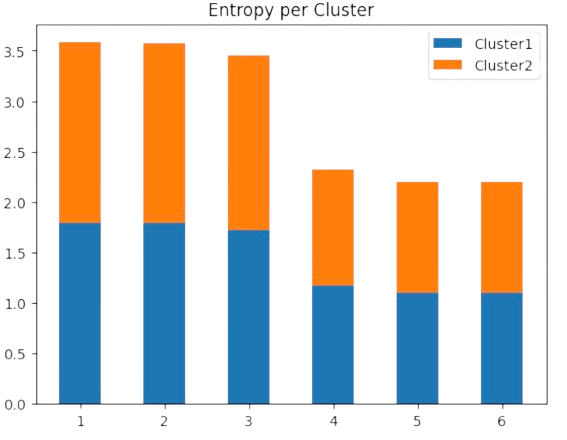
Fig. 2.21 DA as entropy minimization in the exercise example.#
However, as we show in Fig. 2.22 in the motivating example for \(k=3\) clusters, the final maximal entropy per cluster is around \(4-5\) bits (i.e. \(\log 102 = 4.62\) nats). This indicates that the data is not well quantized with \(k=3\) centers.
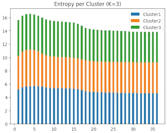
Fig. 2.22 DA as entropy minimization the motivating example (K=3).#
However, as we show in Fig. 2.23 in the motivating example for \(k=3\) clusters, the final maximal entropy per cluster is around \(5\) bits (i.e. \(\log 201 = 5.30\) nats). This indicates that the data is better quantized with \(k=2\) centers: we get (nearly) the same entropy with less centers!
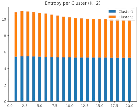
Fig. 2.23 DA as entropy minimization the motivating example (K=2).#
Actually, the new centers are \(\mathbf{c}_1=[0,-1]^T\) and \(\mathbf{c}_2=[0,2]^T\) (see Fig. 2.24).
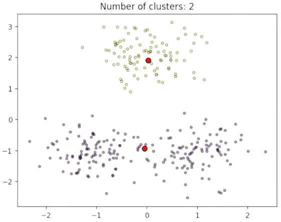
Fig. 2.24 Clusters and estimated prototypes in \(\mathbb{R}^2\) (K=2).#
As a result, entropy is crucial for the interpretation of clustering problems!
2.5. SoftMax for Graph Matching#
2.5.1. SoftMaxing#
2.5.1.1. Continuation Methods#
Back to the graph matching problem or MCS (Maximum Common Subgraph), we have formulated it in discrete terms via SA:
The search space \({\cal P}\) is the set of binary matrices \(\mathbf{M}\in\{0,1\}^{m\times n}\) whose rows and columns have a unique \(1\). When \(m=n\) we have that the search space is the Permuthoedron \(\Pi_n\), i.e. the set of permutation matrices.
SA explores the search space via random walks that eventually hit the global maximum under a slow annealing schedule. Each iteration takes \(O(n^4)\) for evaluating the quadratic cost function \(F(\mathbf{M})\).
We have seen that central clustering can be posed, however, in continuous terms via DA:
The search space is \(\mathbb{R}^d\times {\cal P}\): we have to jointly find \(k\) centers \(\mathbf{c}_i\in\mathbb{R}^d\) and a binary matrix \(\mathbf{M}\in\{0,1\}^{m\times k}\) indicating how the \(m\) points \(\mathbf{x}_a\in\mathbb{R}^d\) are assigned to the most probable cluster.
DA decouples the optimization of the Free energy \(F({\cal C},\mathbf{M})\): given a high-entropic (almost uniform) initial assignment we alternate expectation (update the assignments while the centers are fixed) and update the centers. Each iteration takes \(O(m\times k)\) and it allows faster annealing schedules.
Remember that DA’s success relies on the possibility of evaluating \(Z\) (the Gibbs partition function) thanks to the independence assumption: points are assumed to be independently assigned to any cluster.
In the Gurobi framework , for optimization, where graph matching is seen as a Maximmum Clique, many combinatorial algorithm share the following features with DA:
Transforming the original discrete problem into a continuous one.
Optimize the objective function in the continuous space by means of a polynomial method.
Revert the result to the discrete space through a clean-up heuristic.
These methods are called continuation method.
2.5.1.2. SoftMax operator#
In 1996, Steven Gold and Anand Rangarajan exploited the following simple algorithm for finding the maximum element in a list of numbers:
Algorithm 2.3 (Soft Maximum)
Inputs A list of elements \(L=[X_1,\ldots,X_m]\) with \(X_i\in\mathbb{R}\), \(\beta_0>0\)
Outputs \(m_i>0\) if \(X_i=\max_{L}\) and \(0\) otherwise.
Initialize \(\beta\leftarrow \beta_0\)
while \(\beta < \beta_f\):
for \(i=1,\ldots, m\):
\(m_i\leftarrow \exp(\beta X_i)\)
for \(i=1,\ldots, m\):
\(m_i\leftarrow \frac{m_i}{\sum_{i=1}^m m_i}\)
Increase \(\beta\)
return \(\{m_i\}\) where \(\sum_{i=1}^m m_i=1\)
This algorithm is equivalent to give the \(\{m_i\}\) which maximize \(\sum_{i=1}^m m_iX_i\), now formulated in continuous terms via the control parameter \(\beta>0\). This is the softmax operator:
which is the classical mechanism to select class-membership in the last layer of a neural network!
We show this mechanism in Fig. 2.25. As we increase \(\beta\), the \(m_i\) corresponding to the maximum \(X_i\) (note that there may be many maximal values) tend to \(1\), whereas the \(m_i\) for the non-maximal values drop to \(0\). In the neural-network jargon, this mechanism is dubbed as winner takes all or WTA.
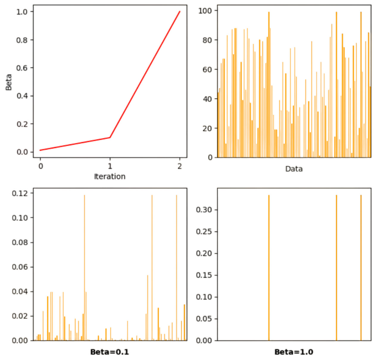
Fig. 2.25 Softmaxing a list of real-valued elements.#
2.5.2. Graduated Assignment#
2.5.2.1. Linear Assignment#
Linear Assignment (LA) is polinomial problem with many applications in Computer Science and AI. Given a bipartite graph \(G=(V,E)\) where: a) \(V = V_1\cup V_2\),\(V_1\cap V_2=\emptyset\) is a vertex partition and b) \(E=V_1\times V_2\), i.e. there are only edges between \(V_1\) and \(V_2\). In addition, the graph is weighted since we are given a matrix of variables \(\mathbf{X}\in\mathbb{R}^{m\times n}\), with \(m=|V_1|\), \(n=|V_2|\), where \(\mathbf{X}_{ai}\) measures the affinity between \(i\in V_1\) and \(j\in V_2\) and its meaning depends on the problem (compatibility between processes and CPUs, local similarity between points of two shapes, etc).
The discrete (original) version of LA is kind of obvious:
In other words, LA is the linear version of QAP where \(\mathbf{X}\) is real-valued instead of being an adjacency matrix. Concerning the search space, if \(m=n\) then \({\cal P}=\Pi_n\) space is the Permuthoedron. However, it is not in NP and actually it can be solved in \(O(n^3)\) with the so called Hungarian algorithm.
However, herein we are going to introduce the soft/continuous version which is basically an extension of SoftMax incorporating:
Continuous assingments. Instead of \(\mathbf{M}\in \{0,1\}^{m\times n}\) we have \(\mathbf{M}\in [0,1]^{m\times n}\).
Two-way constraints. Each \(i\in V_1\) has a probability of being assigned to \(a\in V_2\) and viceversa. Therefore:
i.e. our search space is a matricial generalization of the (vectorial) simplex:
Actually, if \(m=n\) the search space is not the Permuthoedron \(\Pi_n\) but the Birkhoff polytope \(\mathbb{B}_n\). In matricial terms, \(\mathbb{B}_n\) is the set of doubly stochastic matrices (matrices whose rows and columns add \(1\)). In this regard, remember that \(\Pi_n\subset \mathbb{B}_n\) since every permutation matrix is doubly stochastic. Therefore, the vertices of the Birkhoff polytope are the elements of \(\Pi_n\) (solutions to the discrete problem) but during the resolution of the problem continuous solutions lying in the edges and sides of the polytope are allowed.
Algorithmically, the SoftLA needs to enforce the two-way constraints in every iteration as follows:
Algorithm 2.4 (SoftLA)
Inputs Affinity matrix \(\mathbf{X}\in\mathbb{R}^{m\times n}\), \(\beta_0>0\)
Outputs \(\mathbf{M}^{\ast}\) maximal assignment.
Initialize \(\beta\leftarrow \beta_0\)
while \(\beta < \beta_f\):
\(\mathbf{M}_{ai}\leftarrow \exp(\beta \mathbf{X}_{ai})\)
\(\mathbf{M}\leftarrow\text{Sinkhorn}(\mathbf{M})\)
Increase \(\beta\)
return \(\mathbf{M}^{\ast}\) optimal doubly-stochastic matrix.
where \(\text{Sinkhorn}(\mathbf{M})\) is an iterative row-col normalization process which converges to a stochastic matrix:
Algorithm 2.5 (Sinkhorn)
Inputs Exponential assignment matrix: \(\mathbf{M}=\exp(\beta\mathbf{X})\)
Outputs \(\mathbf{M}\) doubly-stochastic matrix.
\(t\leftarrow 0\)
convergence\(\leftarrow\) False
while \(\neg\)convergence:
\(\mathbf{M}^{old}_{ai}\leftarrow \mathbf{M}_{ai}\)
for \(a=1,2,\ldots,m\) (Normalize rows)
\(\mathbf{M}_{ai}\leftarrow \frac{\mathbf{M}_{ai}}{\sum_{i=1}^n \mathbf{M}_{ai}}\)
for \(i=1,2,\ldots,n\) (Normalize cols)
\(\mathbf{M}_{ai}\leftarrow \frac{\mathbf{M}_{ai}}{\sum_{i=a}^m \mathbf{M}_{ai}}\)
\(t\leftarrow t + 1\)
convergence = \((t>t_{max})\) or \((\sum_{ai}|\mathbf{M}_{ai}- \mathbf{M}^{old}_{ai}|\le\epsilon )\)
return \(\mathbf{M}\) doubly-stochastic matrix.
Interestingly, the structure of \(\text{SoftLa}\) is rather simple and essentially is the similar to that of \(\text{SoftMax}\) but for matrices, taking \(O(n^2)\) instead of \(O(n^3)\) as the Hungarian algorithm.
In Fig. 2.26 we show how \(\text{SoftLa}\) solves a problem in a couple of iterations
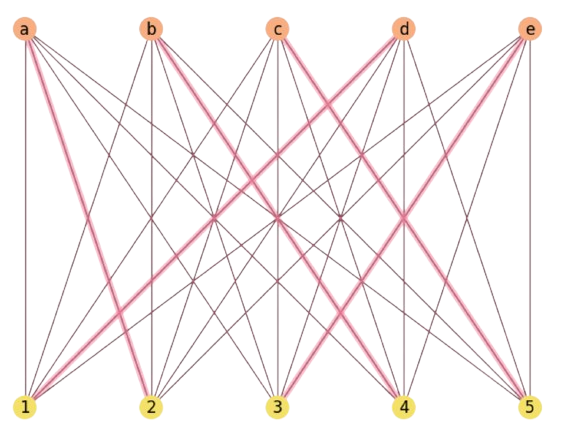
Fig. 2.26 SoftLA solution for a \(m=n=5\) instance with random costs.#
Note that:
The general initialization is \(\mathbf{M}^0=\mathbf{1}^T\mathbf{1}+ \epsilon\mathbf{I}\), i.e. the matrix of ones with a slight perturbation: \(\mathbf{M}^0_{ai}=1+\epsilon\). This initialization is known as baricenter or neutral.
In the above example, \(\mathbf{X}\) is drawn from \(n\times n\) random integers between \(0\) and \(n^2-1\).
The role of \(\text{Sinkhorn}\) is to enforce the two-way constraints and sometimes it may lead to a very entropic doubly-stochastic matrix as we show in the following exercise.
Exercise. Prove that applying \(\text{Sinkhorn}\) to the exponentiation of the above matrix converges to a maximum entropy assignment. Do not use \(\beta\). Explain why.
\( \mathbf{X}= \begin{bmatrix} x & x+\epsilon\\ x-\epsilon & x\\ \end{bmatrix} \)
A priori, it seems that the optimal assignment is \((a=1)\rightarrow (i=2)\) and \((a=2)\rightarrow (i=2)\) but this is not possible due to the two-way constraint. Let us apply the exponential:
\( \mathbf{M}= \begin{bmatrix} e^x & e^{x+\epsilon}\\ e^{x-\epsilon} & e^x\\ \end{bmatrix} \)
Row normalization makes things independent of \(x\):
\( \begin{align} \mathbf{M} &= \begin{bmatrix} \frac{e^x}{e^x + e^{x+\epsilon}} & \frac{e^{x+\epsilon}}{e^x + e^{x+\epsilon}}\\ \frac{e^{x-\epsilon}}{e^x + e^{x-\epsilon}} & \frac{e^x}{e^x + e^{x-\epsilon}}\\ \end{bmatrix} =\begin{bmatrix} \frac{1}{1 + e^{\epsilon}} & \frac{e^{\epsilon}}{1 + e^{\epsilon}}\\ \frac{e^{-\epsilon}}{1 + e^{-\epsilon}} & \frac{1}{1 + e^{-\epsilon}}\\ \end{bmatrix} \end{align} \)
Column normalization:
\( \begin{align} \mathbf{M}_{:1} &= \frac{1}{1 + e^{\epsilon}} + \frac{e^{-\epsilon}}{1 + e^{-\epsilon}} = \frac{(1 + e^{-\epsilon})+e^{-\epsilon}(1 + e^{\epsilon})}{(1 + e^{\epsilon})(1 + e^{-\epsilon})} = \frac{(1 + e^{-\epsilon}) + (1 + e^{-\epsilon})}{(1 + e^{\epsilon})(1 + e^{-\epsilon})} = \frac{2}{1 + e^{\epsilon}}\\ \mathbf{M}_{:2} &= \frac{e^{\epsilon}}{1 + e^{\epsilon}} + \frac{1}{1 + e^{-\epsilon}} = \frac{e^{\epsilon}(1 + e^{-\epsilon}) + (1 + e^{\epsilon})}{(1 + e^{\epsilon})(1 + e^{-\epsilon})} = \frac{(1 + e^{\epsilon}) + (1 + e^{\epsilon})}{(1 + e^{\epsilon})(1 + e^{-\epsilon})} = \frac{2}{1 + e^{-\epsilon}} \end{align} \)
\( \begin{align} \mathbf{M} &= \begin{bmatrix} \frac{\mathbf{M}_{a1}}{\mathbf{M}_{:1}} & \frac{\mathbf{M}_{a2}}{\mathbf{M}_{:2}} \\ \frac{\mathbf{M}_{b1}}{\mathbf{M}_{:1}} & \frac{\mathbf{M}_{b2}}{\mathbf{M}_{:2}} \\ \end{bmatrix} = \begin{bmatrix} \frac{1}{1 + e^{\epsilon}}:\frac{2}{1 + e^{\epsilon}} & \frac{e^{\epsilon}}{1 + e^{\epsilon}}:\frac{2}{1 + e^{-\epsilon}}\\ \frac{e^{-\epsilon}}{1 + e^{-\epsilon}}:\frac{2}{1 + e^{\epsilon}} & \frac{1}{1 + e^{-\epsilon}}:\frac{2}{1 + e^{-\epsilon}}\\ \end{bmatrix} = \begin{bmatrix} \frac{1}{2} & \frac{1}{2}\\ \frac{1}{2} & \frac{1}{2}\\ \end{bmatrix} \end{align} \)
which proves the statement. Why? Well, adding an \(\epsilon\) in one column and subracting it in the opposite column leads to maximal uncertainty wrt the diagonal which is preserved. This is not obvious, and even counter-ituitive, but it is a bit clarified by the removal of \(x\) after row normalization.
2.5.2.2. SoftAssign#
The extension of \(\text{SoftLa}\) to graph matching is almost straight. Now, instead of having a linear cost function, the graph-matching cost function is quadratic in \(\mathbf{M}\) (it is the QAP-Quadratic Assignment Problem). Then, the relaxed QAP becomes
where
\({\cal B}\) is the set of doubly-stochastic matrices of dimension \((m+1)\times (n+1)\), and the Birkhoff polytope or order \(n+1\), i.e. \({\cal B}_{n+1}\), if \(m=n\).
Why an extra dimension? If \(m<n\), for instance, we can only have \(m\) one-to-one assignments and \(n-m\) un-assigned nodes. In order to deal with this, we assume that these un-asigned nodes match a slack or virtual node. Therefore, adding an extra dimension accomodates two virtual nodes (one per graph). Similar reasoning for \(m>n\).
Note that \(\text{SoftLA}\) is just a Deterministic Annealing (DA) applied to linear assignment. If so, one of the driving features of DA is to assume assignment independence, i.e. we may assume that the assignment of \(a\in V\) to \(i\in V'\) is independent of that of another \(a'\in V\) to \(i'\in V'\).
Taylor Expansion. Steven Gold and Anand Rangarajan used a similar principle to approximate the quadratic cost function. Note that \(f(x)\approx f(a) + f'(a)(x-a)\) is the first order Taylor expansion. Then
where
i.e. the derivative of a quadratic function is a linear one! Then, for a fixed \(\mathbf{M}^0\), we have that
i.e. a linear assignment problem. In other words:
\(\mathbf{Q}_{ai}=\sum_{b\in V}\sum_{j\in V'}\mathbf{M}_{bj}\mathbf{X}_{ab}\mathbf{Y}_{ij}\) works as a temporary affinity matrix for each \(\beta\).
Given \(\mathbf{Q}_{ai}\) we iterate to get the best (maximal) assignment \(\mathbf{M}_{ai}\) for this \(\beta\), i.e. we solve a new assignment problem.
Increase \(\beta\) and start again!
This is the typical decoupled structure of DA problems and it leads to the \(\text{SoftAssign}\) algorithm detailed below.
Algorithm 2.6 (SoftAssign)
Inputs Adjacency matrices \(\mathbf{X}\in\{0,1\}^{m\times m}\), \(\mathbf{Y}\in\{0,1\}^{n\times n}\), \(\beta_0>0\)
Outputs \(\hat{\mathbf{M}}^{\ast}\) (extended) maximal quadratic assignment.
Initialize \(\beta\leftarrow \beta_0\), \(\hat{\mathbf{M}}_{ai}\leftarrow 1+\epsilon\)
while \(\beta < \beta_f\):
\(t\leftarrow 0\)
convergence\(\leftarrow\) False
while \(\neg\)convergence:
\(\hat{\mathbf{M}}^{old}_{ai}\leftarrow \hat{\mathbf{M}}_{ai}\)
\(\mathbf{Q}_{ai}\leftarrow \sum_{b=1}^m\sum_{j=1}^n\mathbf{M}_{bj}\mathbf{X}_{ab}\mathbf{Y}_{ij}\)
\(\mathbf{M}^0_{ai}\leftarrow \exp(\beta \mathbf{Q}_{ai})\)
Expand \(\mathbf{M}^0\rightarrow \hat{\mathbf{M}}^0\)
\(\hat{\mathbf{M}}^0\leftarrow\text{Sinkhorn}(\hat{\mathbf{M}}^0)\)
\(t\leftarrow t + 1\)
convergence = \((t>t_{max})\) or \((\sum_{ai}|\hat{\mathbf{M}}_{ai}- \hat{\mathbf{M}}^{old}_{ai}|\le\epsilon' )\)
Increase \(\beta\)
return \(\hat{\mathbf{M}}^{\ast}\) optimal doubly-stochastic matrix.
Some notes:
If \(m\neq n\) we always assume \(m\le n\), i.e. \(\mathbf{X}\) is the smallest graph.
Given the expanded \(\hat{\mathbf{M}}\) in step \(1\), we implicitly use its \(\mathbf{M}\) \(m\times n\) matrix in steps \(3.2\) and \(3.3\).
In step \(3.4\) we expand explicitly \(\mathbf{M}^0\) by incorporating an additiona row and column of zeros. Note that \(\text{Sinkhorn}\) always needs a \((m+1)\times (n+1)\) matrix if \(m\neq n\)!
Complexity. It is not difficult to see that the complexity of \(\text{SoftAssign}\) is roughtly \(O(n^3)\), or more precisely \(O(|E|n)\), if \(m=n\) and \(|E|\) is the number of edges. Such a complexity is due to step 3.2 (the computation of \(\mathbf{Q}\) which involves the product of 3 matrices).
2.5.2.3. Cleanup#
Remember that continuation methods are solved in the continuum but our original is discrete. Given the \(\text{SoftAssign}\) solution \(\hat{\mathbf{M}}^{\ast}\), which can be very entropic, we must recover the closest discrete matrix (which is not unique, in general). This task is performed by a cleanup heuristic or algorithm like the one detailed below:
Algorithm 2.7 (Cleanup)
Inputs \(\hat{\mathbf{M}}\in[0,1]^{(m+1)\times (n+1)}\) optimal doubly-stochastic matrix
Outputs Closest discrete matrix \(\mathbf{M}\in\{0,1\}^{(m+1)\times (n+1)}\)
yet_asigned \(\leftarrow 0\)
\(\mathbf{M}[a,i]\leftarrow 0\)
\(\epsilon \leftarrow 10^{-6}\)
while yet_asigned\(< m\):
changes_done\(\leftarrow\) False
for \(a\in\{1,2,\ldots,m+1\}\):
candidates \(\leftarrow \emptyset\)
max_row \(\leftarrow \max\:\hat{\mathbf{M}}[a,:]\)
row_capacity \(\leftarrow\) max_row \(- \epsilon\)
for \(i\in\{1,2,\ldots,n+1\}\):
max_col \(\leftarrow \max\;\hat{\mathbf{M}}[i,:]\)
col_capacity \(\leftarrow\) max_col \(- \epsilon\)
if \((\mathbf{M}[a,i]>\)row_capacity\()\) and \((\mathbf{M}[a,i]>\)col_capacity\()\):
candidates \(\leftarrow\) candidates \(\cup \{i\}\)
if \(|\)candidates\(|\)>0:
max_val \(\leftarrow\) \(\max \mathbf{M}[a,\)candidates\(]\)
selection \(\leftarrow\) \(\arg\max\) \(\mathbf{M}[a,\)candidates\(]\)
col \(\leftarrow\) candidates[selection]
yet_assigned \(\leftarrow\) yet_assigned + 1
\(\mathbf{M}[a,\)col\(]\leftarrow\) 1
\(\mathbf{M}[a,:]\leftarrow-\infty\)
\(\mathbf{M}[:,col]\leftarrow-\infty\)
changes_done \(\leftarrow\) True
if \(\neg\) changes_done:
break
return \(\mathbf{M}\) binary matrix.
The algorithm, basically a greedy version of the Hungarian algorithm, proceeds as follows:
Steps 2.1-2.4. For every row \(a\), we build a list of candidates keeping track of both the row and col capacities.
Step 2.5. If the list of candidates is not empty, we proceed to get the best of them (step 5.5) and then we proceed to exclude the corresponding row and column (steps 5.6 and 5.7).
This takes \(O(n^2)\) and could be replaced by a run of \(\text{SoftLA}\). Remember that if the algorithm finds any match to a slack vertex these machings should be cleared.
Results. Coming back to the Aspirin Isomorphism, we use the setting recommended in Gold and Rangarajan’s paper: \(\epsilon = 0.1\), \(\epsilon'=0.5\), \(\beta_0=0.5\), \(\beta_f=10.0\), \(\beta_r=1.075\) and \(I_0=4\), \(I_1=30\), where the last two numbers are the maximal iterations of the internal while loop and \(\text{Sinkhorn}\), respectively.
The result in Fig. 2.27 is nearly perfect and we can claim that Aspirin is isomorphic wrt to a permutation of itself!
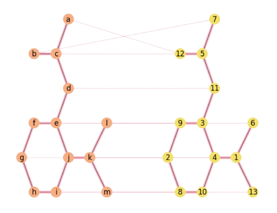
Fig. 2.27 Detecting the Aspirin’s Isomorphism with DA.#
We leave to the practice lessons the extension of the algorithm for incorporating both node and edge attributtes.
2.6. Appendix#
2.6.1. Independence#
Statistical independence. It is well known that two random variables \(A\) and \(B\) are independent iff:
Or, in other words, applying the Bayes theorem we have that \(A\) and \(B\) are independent iff
In other words:
Independence implies factorizing the joint distribution \(p(A,B)\)
\(A\) and \(B\) are indendent if the knowledge of one of them does not influence the probability of the other, i.e. \(p(A|B)=p(A)\) and \(p(B|A)=p(B)\).
Marginalization. Alternatively, we may define statistical independence by checking the marginal probabilities. Let \(a_1,a_2,\ldots,a_m\) the discrete values of \(A\) and \(b_1,b_2,\ldots,b_n\) similarly for \(B\). Then:
Then, \(A\) and \(B\) are independent if we can write a joint distribution as the product of two marginal distributions:
Let us practice a bit this concept in the following exercise.
Exercise. Given the above table representing the joint distribution of two discrete random variables \(A\) and \(B\), determine where they are indepedent or not. a) Usign the marginals. b) Using the conditional probabities.
\(
\begin{aligned}
\begin{array}{c|ccc}
& B=b_1 & B=b_2 & B=b_3 \\
\hline
A=a_1 & 0.1 & 0.2 & 0.3\\
A=a_2 & 0.1 & 0.2 & 0.1\\
\hline
\end{array}
\end{aligned}
\)
a) First all, note that \(\sum_{a_i,b_j}p(A=a_i,B=b_j)=1\). Now, let us compute the marginals summing the rows for \(A\) and the columns for \(B\):
\(
\begin{align}
p(A=a_1) &= \sum_{b_j}p(A=a_1,B=b_j)=0.1 + 0.2 + 0.3 = \mathbf{0.6}\\
p(A=a_2) &= \sum_{b_j}p(A=a_2,B=b_j)=0.1 + 0.2 + 0.1 = \mathbf{0.4}\\
p(B=b_1) &= \sum_{a_i}p(A=a_i,B=b_1)=0.1 + 0.1 = \mathbf{0.2}\\
p(B=b_2) &= \sum_{a_i}p(A=a_i,B=b_2)=0.2 + 0.2 = \mathbf{0.4}\\
p(B=b_3) &= \sum_{a_i}p(A=a_i,B=b_3)=0.3 + 0.1 = \mathbf{0.4}\\
\end{align}
\)
Now we check independence:
\(
\begin{align}
p(A=a_1,B=b_1) &=0.1\neq p(A=a_1)p(B=b_1) = \mathbf{0.6}\times\mathbf{0.2}=0.12\\
p(A=a_1,B=b_2) &=0.2\neq p(A=a_1)p(B=b_2) = \mathbf{0.6}\times\mathbf{0.4}=0.24\\
p(A=a_1,B=b_3) &=0.3\neq p(A=a_1)p(B=b_3) = \mathbf{0.6}\times\mathbf{0.4}=0.24\\
p(A=a_2,B=b_1) &=0.1\neq p(A=a_2)p(B=b_1) = \mathbf{0.4}\times\mathbf{0.2}=0.08\\
p(A=a_2,B=b_2) &=0.2\neq p(A=a_2)p(B=b_2) = \mathbf{0.4}\times\mathbf{0.4}=0.16\\
p(A=a_2,B=b_3) &=0.1\neq p(A=a_2)p(B=b_3) = \mathbf{0.4}\times\mathbf{0.4}=0.16\\
\end{align}
\)
However, note that in all cases \(p(A=a_i,B=b_j)\approx p(A=a_i)p(B=b_j)\).
b) Now, we can compute the conditional probabilities using the Bayes theorem: \(p(A=a_i|B=b_j)=p(A=a_i,B=b_j)/p(B=b_j)\)
\(
\begin{aligned}
\begin{array}{c|ccc}
& B=b_1 & B=b_2 & B=b_3 \\
\hline
p(A=a_1|B=b_j) & \frac{0.1}{0.2}=0.5 & \frac{0.2}{0.4}=0.5 & \frac{0.3}{0.4}=0.75\\
p(A=a_2|B=b_j) & \frac{0.1}{0.2}=0.5 & \frac{0.2}{0.4}=0.5 & \frac{0.1}{0.4}=0.25\\
\hline
& \sum = 1 & \sum = 1 & \sum=1\\
\end{array}
\end{aligned}
\)
and \(p(B=b_j|A=a_i)=p(A=a_i,B=b_j)/p(A=a_i)\)
\(
\begin{aligned}
\begin{array}{c|ccc|c}
& p(B=b_1|A=a_i) & p(B=b_2|A=a_i) & p(B=b_3|A=a_i) \\
\hline
A=a_1 & \frac{0.1}{0.6}=0.17 & \frac{0.2}{0.6}=0.33 & \frac{0.3}{0.6}=0.5 & \sum = 1\\
A=a_2 & \frac{0.1}{0.4}=0.25 & \frac{0.2}{0.4}=0.5 & \frac{0.1}{0.4}=0.25 & \sum = 1\\
\hline
\end{array}
\end{aligned}
\)
Note that the conditional probabilities adds \(1\) wrt the “influenced” variable, i.e.
\(
\forall a_i: \sum_{b_j} p(A=a_i|B=b_j)= 1\;\text{and}\;
\forall b_j: \sum_{a_i} p(B=b_j|A=a_i)= 1
\)
2.6.2. Entropy#
This is the first point in the subject where we talk about Information Theory, the main auxiliary maths behind this course. In this regard, we refer you to the author’s book on the subject.
2.6.2.1. Definition and properties#
The above exercise reveals one esential property of DA: we cannot converge without keeping the maximizing the entropy. But, what is entropy?
Entropy is the ultimate measure of uncertainty defined by Shannon as follows:
Given a discrete random variable \(X\), with possible values \(\{x_1,\ldots,x_n\}\), its entropy is given by:
Similarly, we can express entropy in terms of the probabilities of the discrete events \(p_i=p(X=x_i)\), i.e.
Then, we have the following properties:
\(H\) is continuous, concave and non-negative in \(p_i\).
If all the \(p_i\) are equally likely, i.e. \(p_i=1/n\), then entropy is maximal for this \(n\) and equal to \(\log n\). The larger \(n\) the larger the uncertainty of the equally likely events.
If we have \(\log_2\) entropy is measured in bits, whereas if it is \(\ln\) it is measured in nats.
Since \(E(f(x))=\sum_x x\cdot f(x)\) is the expectation of \(f(x)\), then entropy is the expectation of the logarithm.
Entropy of Bernouilli. An interesting example is the measure of the entropy of \(X\sim \text{Bernouilli}(p)\).
\(X\) has value \(x=1\) with probability \(p(X=1)=p\) and \(x=0\) with probability \(p(X=0)=q=1-p\). Then:
Therefore, the maximal entropy (uncertainty) of a Bernouilli variable is when \(p=q=1/2\) (for instance the probability of a fair coin):
which is \(\log_2 2=1\) bits as we can see in Fig. 2.28. Note that the function is concave wrt \(p\). Minimal entropy is achieved at the two extreme points: \(p=0\) and \(p=1\), where the uncertainty is minimal (completely biased coin).
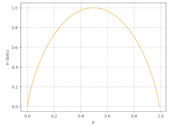
Fig. 2.28 Entropy of Bernouilli wrt \(p\).#
2.6.2.2. Entropy and Coding#
The relationship between entropy and codelength is key to understand why entropy measures information content.
The Morse code follows the principle of assigning less number of bits to more frequent letters than to less frequent ones. Herein, the bits are clear: \(0\) for the dits “.” and \(1\) for the dash “.”. For instance, following the frequencies of letters in English, the shorter “codewords” are those for \(E=.\) and \(T=-\). The longer ones are those for the digits \(0-9\) (five bits all of them). The table below shows those lengths and probabilities.
Note that, due to traditional reasons it is not always happening that shorter codes correspond to highest frequencies (probabilities) but this is the global trend.
Of course, each message should have a space ‘ ‘ between letters in order to be decoded properly. For instance: “……-.. .-.. — .– — .-. .-.. -..” means H E L L O W O R L D in Morse.
Codes and Trees. One interesting way of characterizing codes (binary codes in particular) is to try to put the symbols to code in a tree. See for instance Fig. 2.29, where the root is marked as “#’. We point out the following:
Decoding means navigating through the tree top-to-bottom, making decisions (dit or slash for binary codes), i.e. building a “path”, until the desired symbol is reached. Such a path is the “codeword”.
The codeword length \(l_i\) is the number of decision taken to decode it, i.e. the depth of the symbol in the tree.
A code is comma-like if all the symbols are placed at the leaves of the tree. This is clearly not the case of Morse.
A code is prefix-like if any symbol is preceeded by a unique sequence of other codes (the prefix). For instace, to decode “O” in Morse, we should decode “T” and “M”. Thus, the prefix of “O” is “TM”.
In the Morse code few letters are placed at the leaves of tree. Notably, they are the ones with the largest codeword lengths. Herein, we follow the recipe that assigning less frequent letters to deeper levels of the tree. The purpose of such strategy is twofold: (a) saving storage space, and (b) fast decoding.
Expected codelength. Suppose that we have \(n\) letters, each one with frequency \(p_i\) and codelenth \(l_i\), \(i=1,\ldots,n\). Then, the expected codelength is
For the Morse code, \(E_{Morse}(l)=3.0794539323542267\). Now, the tree in Fig. 2.29 is built under the constraint of placing more probable letters in the top of the (binary) tree. In other words, we may assume that
If so, \(E(l)\approx H(p_1,p_2,\ldots,p_n)\) since
Then
Roughly speaking, the expected codelegth matches entropy!
More precisely, for comma-like codes we have \(E(l)\le H(p_1,p_2,\ldots,p_n)\). Although Morse is not comma-like it satisfies this bound since \(E_{Morse}(l) = 3.0794539323542267\le H_{Morse} = 4.713102340698242\).
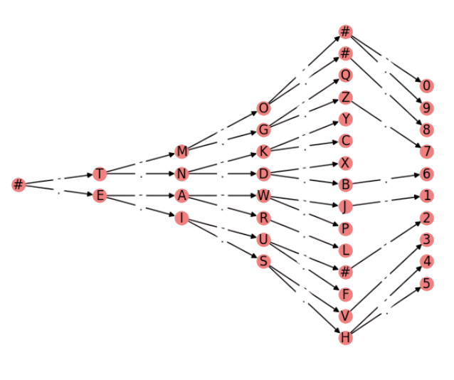
Fig. 2.29 Decoding tree for the Morse code.#
Huffman Codes. As an alternative code, herein we highlight a prefix code (no code is the prefix of another). Prefix codes are easily decodable and, in addition, they allow us (by definition) to suppress the space “ “ between words (see the Table below).
For instance, the Huffman code for HELLOW WORLD is
Concerning \(E_{Huffman}(l)\) and \(H_{Huffman}=\), they are identical: \(4.7\). See the encoding tree in Fig. 2.30
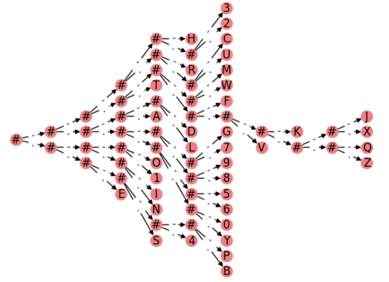
Fig. 2.30 Decoding tree for the Huffman code of the Morse frequencies.#
Finally, this code is not only useful for English but for any laguage such as Chinese.
2.6.2.3. Joint vs Conditional entropy#
Entropy is defined for any (discrete) probability function, and in particular for the joint probability. Thus, if \(A\) and \(B\) are two discrete variables with respective values \(a_1,\ldots, a_m\) and \(b_1,\ldots,b_n\) and does exists the probability \(p(A,B)\), the joint entropy \(H(A,B)\) is defined as follows:
Remember that the Bayes theorem leads to \(p(A,B)=p(A|B)p(B)=p(B|A)p(A)\). As a result, we may define entropies for \(p(A|B)\) and \(p(B|A)\), i.e. conditional entropies.
Remember that entropy is an expectation, then
is the entropy of the conditional expectation of \(A\) wrt \(B=b_j\). Now, if we average this quantity wrt all values \(b_j\), we have that the conditional entropy is given by following weigthed sum:
and similarly for \(H(B|A)\). Actually we have several properties linking conditional entropies and joint entropies:
Zero-value: \(H(A|B)=0\) if the value of \(A\) is completely determined by \(B\). In other words, \(H(A|B)\) measures how much uncertainty adds \(B\) to \(A\). Then, if \(p(A|B)=1\) it is expected that knowing \(B\) is the same as knowing \(A\) itself.
Independence: \(H(A|B)=H(A)\) and \(H(B|A)=H(A)\) iff \(A\) and \(B\) are independent, as it happens with \(p(A|B)=p(A)\) and \(p(B|A)=p(A)\).
Chain rule: the conditional entropies can be derived from the joint entropy \(H(A,B)\) by subtracting the entropy of the conditioning variable:
Exercise. Given the discrete random variales \(A\) and \(B\), in the previous exercise: a) determine the joint entropy and b) the conditional entropies. c) Interpret what is the uncertainty added or removed by each variable wrt to the other and the uncertainty removed from the joint entropy. d) Are \(A\) and \(B\) independent attending to their entropies?
a) First all, for the joint entropy we need the joint distribution:
\(
\begin{aligned}
\begin{array}{c|ccc}
& B=b_1 & B=b_2 & B=b_3 \\
\hline
A=a_1 & 0.1 & 0.2 & 0.3\\
A=a_2 & 0.1 & 0.2 & 0.1\\
\hline
\end{array}
\end{aligned}
\)
\(
\begin{align}
H(A,B) &= -\sum_{a_i}\sum_{b_j}p(A=a_i,B=b_j)\log p(A=a_i,B=b_j)\\
&= -[3(0.1\log 0.1) + 2(0.2\log 0.2) + 0.3\log 0.3]\\
&= \mathbf{1.695}\;\text{nats}\;.
\end{align}
\)
Note that the maximum entropy (in this case with \(m\cdot n=6\) events) is given when
all events are equiprobable, i.e. \(p(A=a_i,B=b_j)=\frac{1}{m\cdot n}=\frac{1}{2\cdot 3}=\frac{1}{6}\), and it is \(H_{max}(A,B)=\log n = \log 6\)
\(
\begin{align}
H_{max}(A,B) &= -\sum_{a_i}\sum_{b_j}\frac{1}{m\cdot n}\log \frac{1}{m\cdot n}\\
&= -6\cdot \frac{1}{6}\log\frac{1}{6}\\
&= -\log\frac{1}{6}\\
&= -(\log 1 - \log 6)\\
&= \log 6 = 1.791\;\text{nats}\;.
\end{align}
\)
Then \(H(A,B)=1.695\) is pretty close to \(H_{max}(A,B)=1.791\).
b1) For \(H(A|B)\) we need the conditional distribution \(p(A|B)\):
\(
\begin{aligned}
\begin{array}{c|ccc}
& B=b_1 & B=b_2 & B=b_3 \\
\hline
p(A=a_1|B=b_j) & \frac{0.1}{0.2}=0.5 & \frac{0.2}{0.4}=0.5 & \frac{0.3}{0.4}=0.75\\
p(A=a_2|B=b_j) & \frac{0.1}{0.2}=0.5 & \frac{0.2}{0.4}=0.5 & \frac{0.1}{0.4}=0.25\\
\hline
& \sum = 1 & \sum = 1 & \sum=1\\
\end{array}
\end{aligned}
\)
Then, attending to the definition \(H(A|B)=\sum_{b_j}p(B=b_j)H(A|B=b_j)\), we have:
\(
\begin{align}
H(A|B=b_1) &= -\sum_{a_i}p(A=a_i|B=b_1)\log p(A=a_i|B=b_1)\\
&= -(0.5\log 0.5 + 0.5\log 0.5) = 0.693\\
H(A|B=b_2) &= -\sum_{a_i}p(A=a_i|B=b_2)\log p(A=a_i|B=b_2)\\
&= -(0.5\log 0.5 + 0.5\log 0.5) = 0.693\\
H(A|B=b_3) &= -\sum_{a_i}p(A=a_i|B=b_3)\log p(A=a_i|B=b_3)\\
&= -(0.75\log 0.75 + 0.25\log 0.25) = 0.562\\
\end{align}
\)
Then, \(H(A|B)\) is given by a weighted average, where we need the marginals \(p(B=b_j)=[0.2\;0.4\;0.4]\) (see the corresponding exercise):
\(
\begin{align}
H(A|B) &= \sum_{b_j}p(B=b_j)H(A|B=b_j)\\
&= p(B=b_1)H(A|B=b_1) + p(B=b_2)H(A|B=b_2) + p(B=b_3)H(A|B=b_3)\\
&= 0.2\cdot H(A|B=b_1) + 0.4\cdot H(A|B=b_2) + 0.4\cdot H(A|B=b_3)\\
&= 0.2\cdot 0.693 + 0.4\cdot 0.693 + 0.4\cdot 0.562\\
&= \mathbf{0.640}\;.
\end{align}
\)
b2) For \(H(B|A)\) we need the conditional distribution \(p(B|A)\):
\(
\begin{aligned}
\begin{array}{c|ccc|c}
& p(B=b_1|A=a_i) & p(B=b_2|A=a_i) & p(B=b_3|A=a_i) \\
\hline
A=a_1 & \frac{0.1}{0.6}=0.17 & \frac{0.2}{0.6}=0.33 & \frac{0.3}{0.6}=0.5 & \sum = 1\\
A=a_2 & \frac{0.1}{0.4}=0.25 & \frac{0.2}{0.4}=0.5 & \frac{0.1}{0.4}=0.25 & \sum = 1\\
\hline
\end{array}
\end{aligned}
\)
Then, attending to the definition \(H(B|A)=\sum_{a_i}p(A=a_i)H(B|A=a_i)\), we have:
\(
\begin{align}
H(B|A=a_1) &= -\sum_{b_j}p(B=b_j|A=a_1)\log p(B=b_j|A=a_1)\\
&= -(0.17\log 0.17 + 0.33\log 0.33 + 0.5\log 0.5) = 1.013\\
H(B|A=a_2) &= -\sum_{b_j}p(B=b_j|A=a_2)\log p(B=b_j|A=a_2)\\
&= -(0.25\log 0.25 + 0.5\log 0.5 + 0.25\log 0.25) = 1.039\\
\end{align}
\)
Then, \(H(B|A)\) is given by a weighted average, where we need the marginals \(p(A=a_i)=[0.6\;0.4]\) (see the corresponding exercise):
\(
\begin{align}
H(B|A) &= \sum_{a_i}p(A=a_i)H(B|B=a_i)\\
&= p(A=a_1)H(B|A=a_1) + p(A=a_2)H(B|A=a_2)\\
&= 0.6\cdot H(B|A=a_1) + 0.4\cdot H(B|A=a_2)\\
&= 0.6\cdot 1.013 + 0.4\cdot 1.039 \\
&= \mathbf{1.023}\;.
\end{align}
\)
c) As a result \(H(B|A)=\mathbf{1.023}>H(A|B)=\mathbf{0.640}\). This means that \(B\) holds more information about \(A\) than \(A\) holds about \(B\).
Finally, let us compute the individual entropies \(H(A)\) and \(H(B)\):
\(
\begin{align}
H(A) & = -\sum_{a_i}p(A=a_i)\log p(A=a_i)\\
& = -(0.6\log 0.6 + 0.4\log 0.4)\\
& = \mathbf{0.673}\;.\\
H(B) & = -\sum_{b_j}p(B=b_j)\log p(B=b_j)\\
& = -(0.2\log 0.2 + 0.4\log 0.4 + 0.4\log 0.4)\\
& = \mathbf{1.054}\;.\\
\end{align}
\)
Since \(H(A|B)=H(A,B)-H(B)\) and \(H(B|A)=H(A,B)-H(A)\) and \(H(B)>H(A)\) (\(B\) is more uncertain than \(A\)), then \(H(B)\) reduces more the uncertainty of \(H(A,B)\) than \(H(A)\). This explains why \(H(A|B)\ll H(B|A)\).
Let us check the calculus:
\(
H(A|B) = \mathbf{0.640} = 1.695 - 1.054\;\;\text{and}\;\; H(B|A) = \mathbf{1.023} = 1.695 - 0.673\;.
\)
d) Since \(H(A|B)=0.640\approx H(A)= 0.673\) and \(H(B|A)=1.023\approx H(B)=1.054\), we conclude that \(A\) and \(B\) are close to be independent, although they are not. This is consistent with the previous exercise on marginals.
Then, in this exercise we have illustrated how to compute the conditional entropies either directly or through the individual entropies and the joint entropy. However, the key of this exercixse is to interpret correctly what a conditional entropy is: a quantification of how much information has one variable about the other.